Essence of Linear Algebra

10 Apr 2023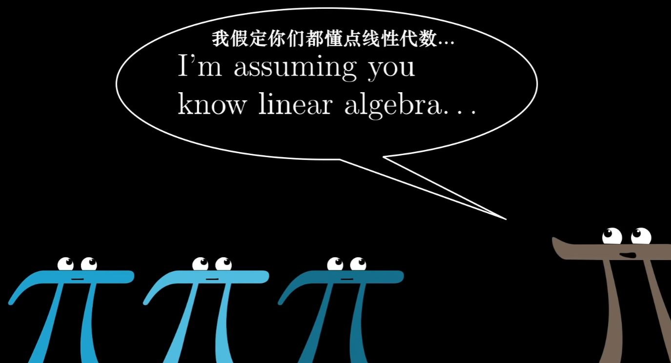

Watch the series here: https://www.bilibili.com/video/BV1ys411472E

The Essence of Linear Algebra

Chapter 1: What is a Vector?

Three Perspectives on Vectors

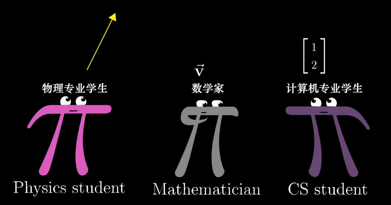
Physics Perspective: A vector is an arrow in space, defined by its length and direction.
Computer Science Perspective: A vector is an ordered list of numbers.
Mathematics Perspective: A vector can be anything, as long as vector addition and scalar multiplication are well-defined.

Vectors in Linear Algebra

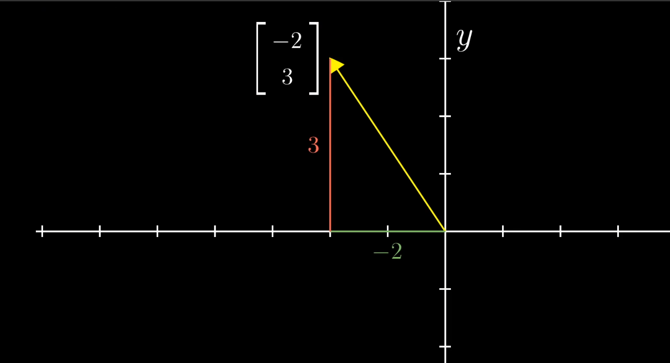
From a geometric standpoint, vectors in linear algebra are arrows originating from the origin of a coordinate system. Their coordinates represent their components along each axis.

(Since vectors almost always start at the origin, we can sometimes think of a vector simply as a point in space—the point where its tip lands.)

Basic Vector Operations

Addition: Visualized using the triangle rule (or parallelogram rule), representing the composition of movements.
Scalar Multiplication: The act of scaling (stretching or compressing) and/or flipping a vector.

Chapter 2: Linear Combinations, Span, and Basis Vectors

Linear Combinations

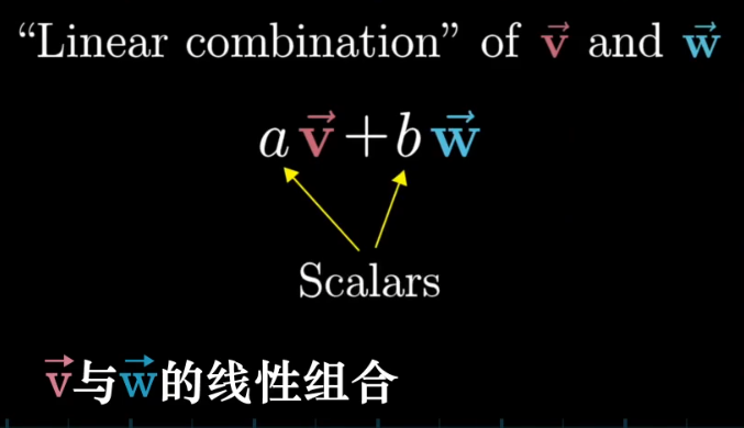
The sum of two scaled vectors is called a linear combination of those vectors.

One way to think about the “linear” part: If you fix one scalar and let the other vary freely, the tips of the resulting vectors will trace a straight line.

Depending on the vectors, their linear combinations can have different outcomes:

In most cases, the linear combinations of two 2D vectors v and w can reach any point in the 2D plane.
In special cases (e.g., if they are collinear or both are zero vectors), they might only span a line or the origin itself.

Span

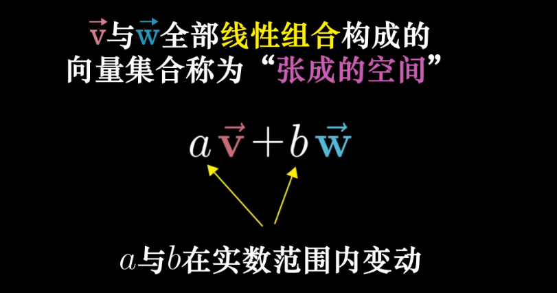
The set of all possible vectors you can reach with a linear combination of a given set of vectors is called the span of those vectors.

Linear Dependence and Independence

Linearly Dependent: A set of vectors is “linearly dependent” if you can remove at least one of them without shrinking the span.
- Alternatively, it means one of the vectors can be expressed as a linear combination of the others.
Linearly Independent: A set of vectors is “linearly independent” if each vector adds a new dimension to the span.

Basis Vectors

A basis of a vector space is a set of linearly independent vectors that spans the entire space.

Chapter 3: Matrices and Linear Transformations

Linear Transformations

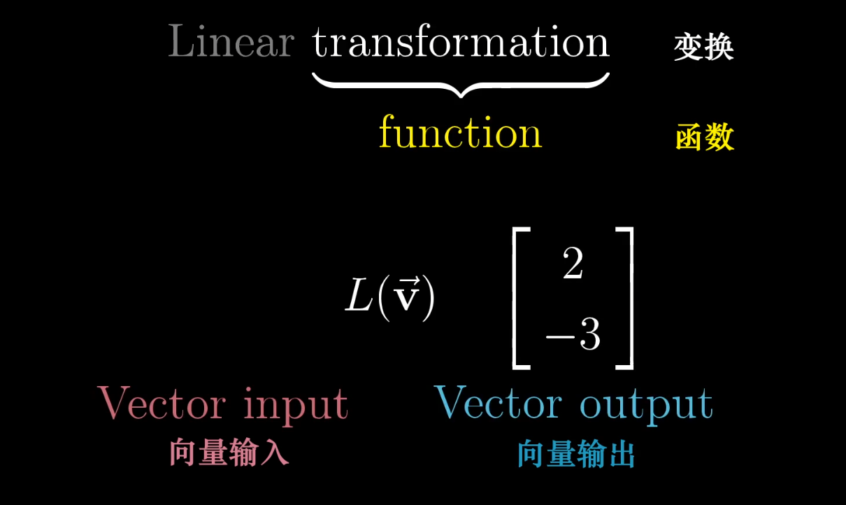
The term “transformation” is essentially another word for “function”; it takes an input and produces an output. Using “transformation” emphasizes the idea of motion, which provides excellent geometric intuition for what happens to vectors.

In linear algebra, a transformation moves all points in a vector space to new locations.

A linear transformation is a special kind of transformation with two properties:

All lines must remain lines after the transformation.
The origin must remain fixed.

Visually, a linear transformation keeps grid lines parallel and evenly spaced, without moving the origin.

The core idea: We only need to track where the basis vectors land. The transformation of any other vector can be described as a linear combination of these transformed basis vectors.

The Geometric Meaning of Matrix-Vector Multiplication

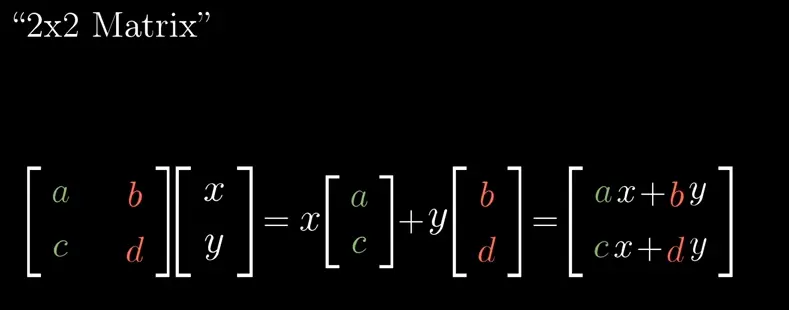
Each column of a matrix represents the coordinates of a transformed basis vector. Multiplying a matrix by a vector (x, y) gives the coordinates of that vector after the transformation.

Whenever you see a matrix, you can interpret it as a specific transformation of space.

Chapter 4: Matrix Multiplication and Composition

A composite transformation is the new linear transformation that results from applying several individual transformations one after another.

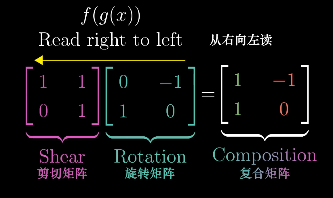
The matrix of a composite transformation is the product of the individual transformation matrices. The product is calculated from right to left, corresponding to the order of application.

Crucially, matrix multiplication is not commutative. Geometrically, this means that changing the order of transformations will generally result in a different final transformation.

Chapter 5: The Determinant

Geometric Meaning of the Determinant

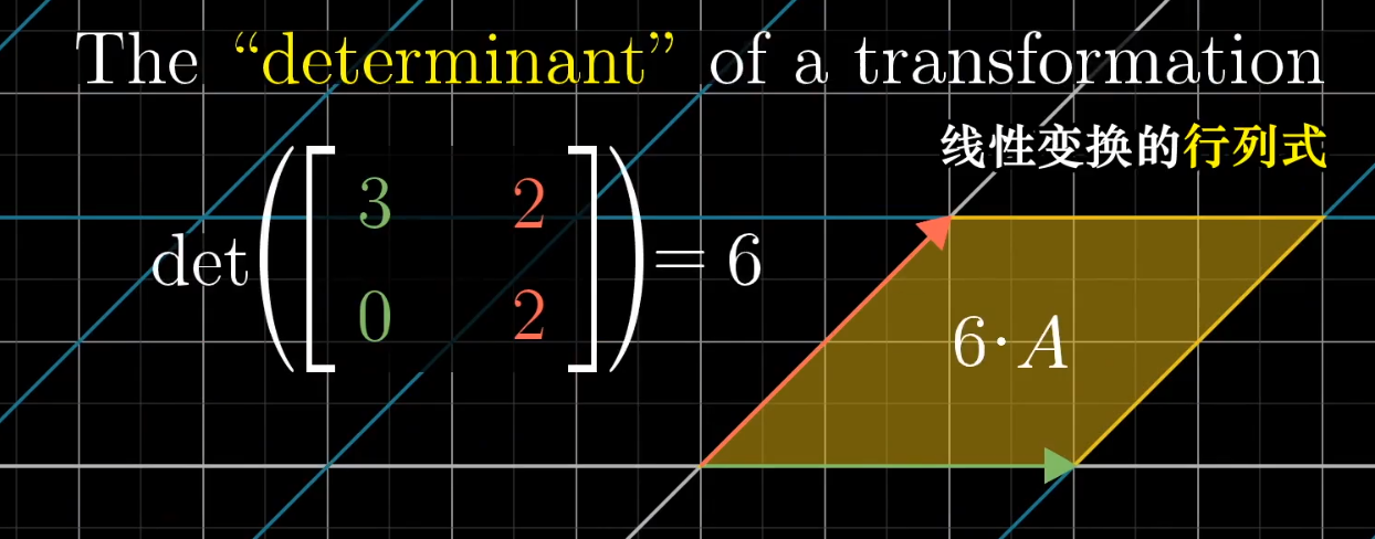
The determinant of a transformation is the factor by which areas are scaled.

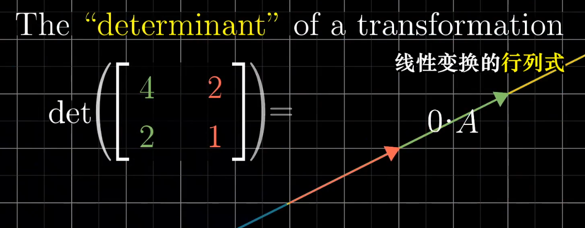
A determinant of zero means the transformation squishes space into a lower dimension (e.g., a plane becomes a line or a point). This is a vital property, as it indicates that the columns of the matrix are “linearly dependent.”

What about a Negative Determinant?

The determinant represents a scaling factor, so why can it be negative? A negative sign indicates that the transformation inverts the orientation of space. The absolute value of the determinant still represents the scaling factor for area.

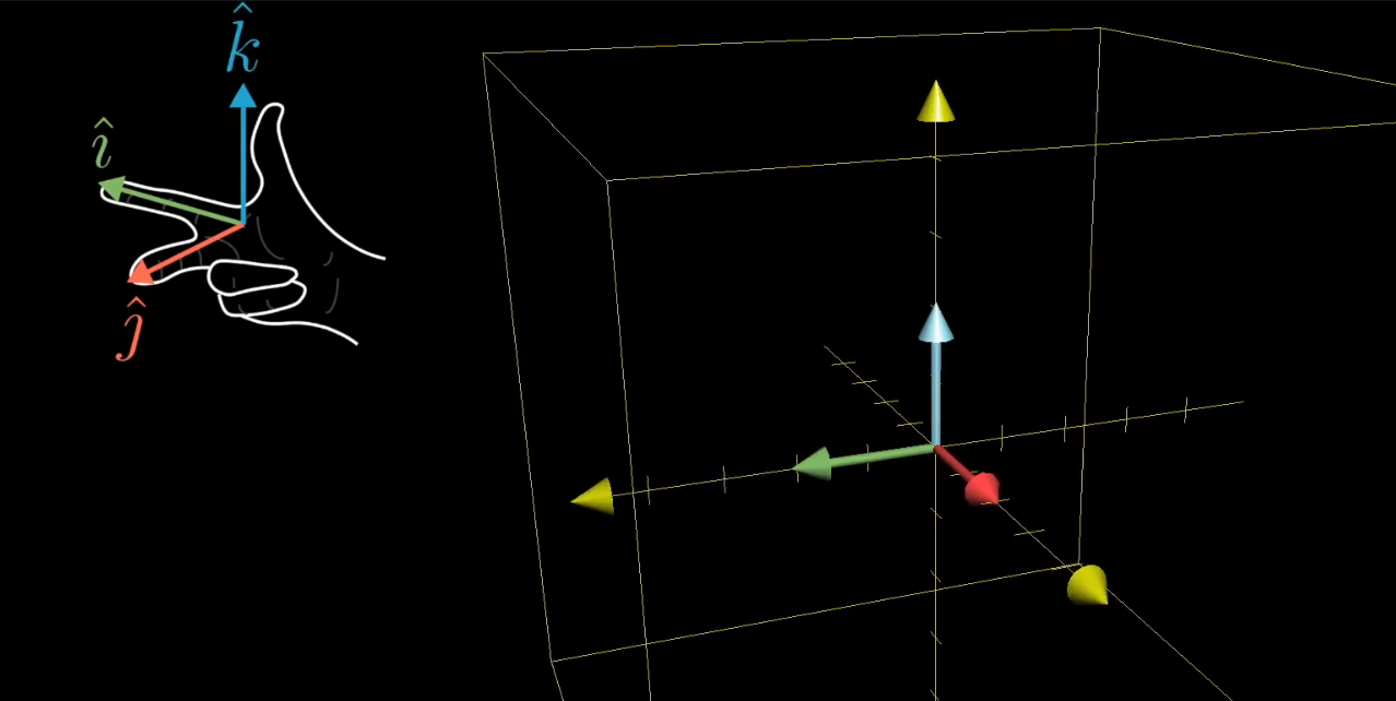
In 3D, a negative determinant means the transformation changes a “right-hand system” into a “left-hand system.”

Chapter 6: Inverse Matrices, Column Space, and Null Space

Solving Systems of Linear Equations

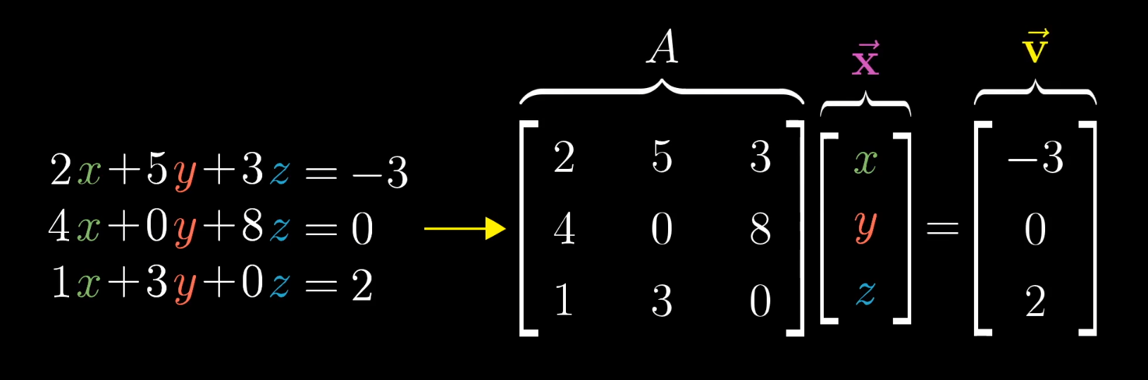
A major application of linear algebra is solving systems of linear equations. We can view a system Ax = v geometrically as searching for an unknown vector x that, after being transformed by matrix A, lands on a known vector v.

When det(A) ≠ 0: The transformation does not reduce the dimensionality of space. This means you can always find a unique x by applying the inverse transformation (A⁻¹) to v.
When det(A) = 0: The transformation squishes space into a lower dimension, and an inverse transformation does not exist. A solution exists only if the target vector v happens to lie within that lower-dimensional output space. If a solution exists, there will be infinitely many, as multiple input vectors x get mapped to the same output vector.

Rank

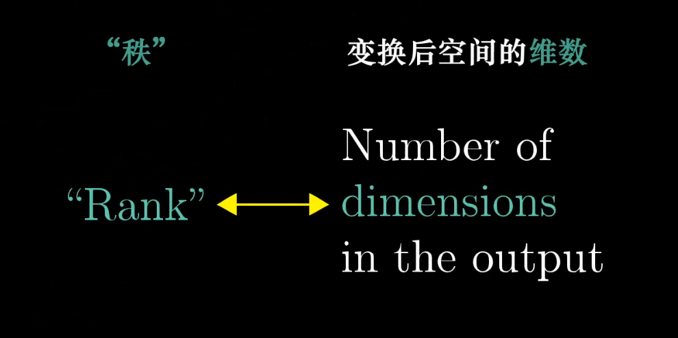
The rank of a transformation is the number of dimensions in the output space. More precisely: The rank is the dimension of the column space.

Column Space

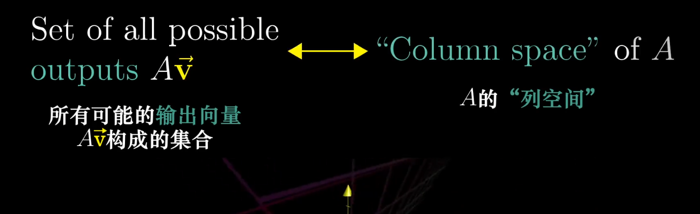
The set of all possible output vectors of a transformation is called its column space.

Since the columns of a matrix tell you where the basis vectors land, the column space is simply the span of the columns of the matrix. The zero vector is always included in the column space, as a linear transformation must keep the origin fixed.

Null Space

The set of all vectors that land on the origin (the zero vector) after a transformation is called the null space (or kernel).

For a full-rank transformation, only the origin itself maps to the origin.
For a non-full-rank transformation, which compresses space, a whole line or plane of vectors can be mapped to the origin, forming the null space.

Chapter 7: Dot Product and Duality

Standard Interpretation of the Dot Product

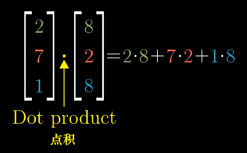
For two vectors of the same dimension, multiply their corresponding components and add the results.

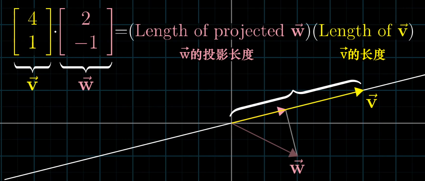
Geometrically, it is the length of the projection of one vector onto the other, multiplied by the magnitude of the other vector.

The Dot Product from a Linear Algebra Perspective

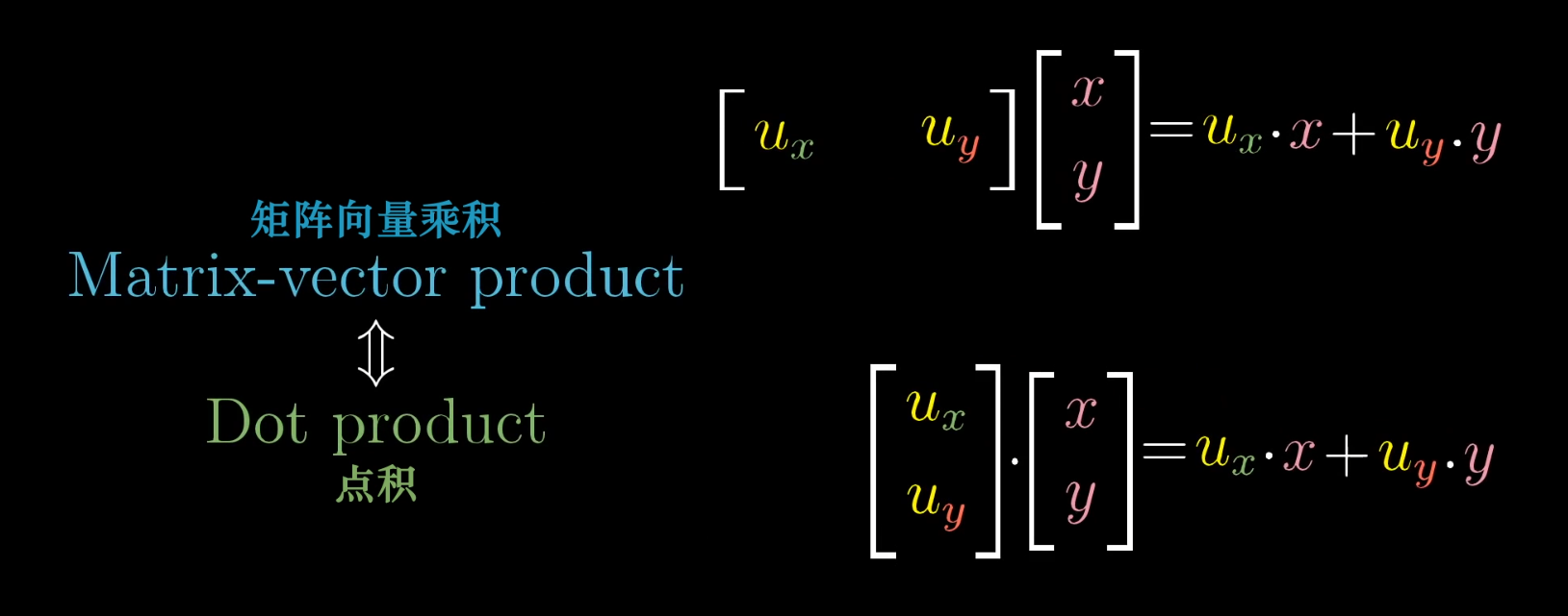
We can think of the dot product with a specific vector as a transformation from a 2D space to a 1D space (the number line).

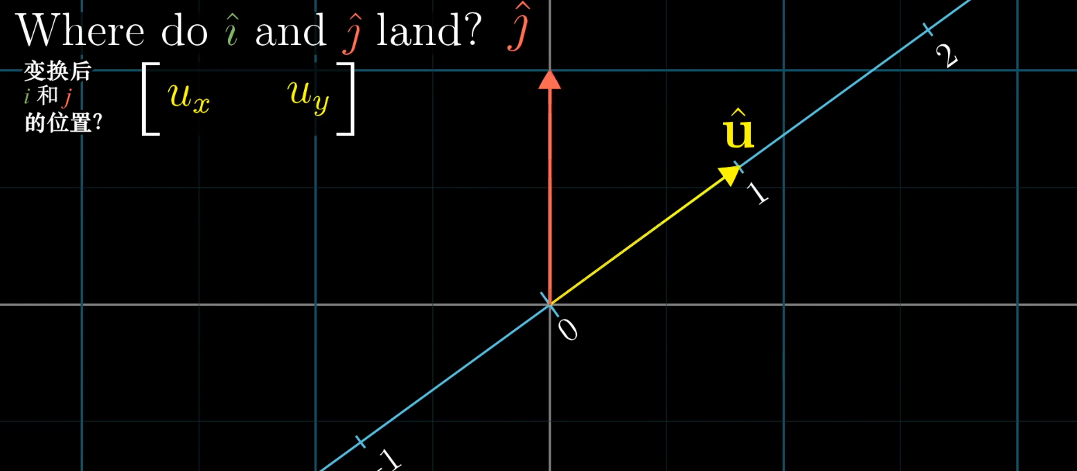
Due to symmetry, the matrix that defines this 2D-to-1D transformation is simply the coordinates of that vector. How cool is that!

Chapter 8: Cross Product

Standard Interpretation of the Cross Product

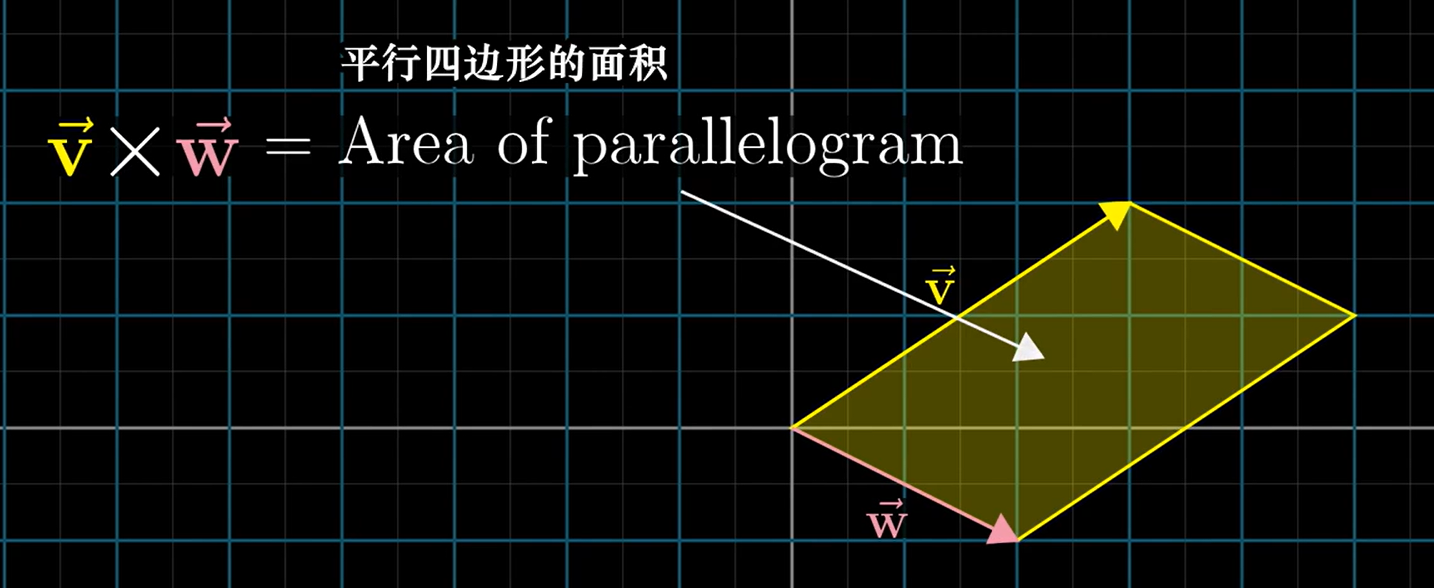
The magnitude of the cross product v × w is the area of the parallelogram formed by the two vectors. Its direction is determined by their relative orientation and the right-hand rule.

For 3D vectors, the cross product yields a new vector that is perpendicular to both v and w. Its magnitude is the area of the parallelogram they form, and its direction follows the right-hand rule.

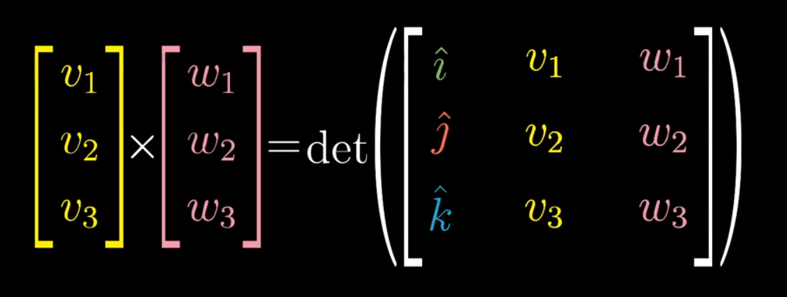
The Cross Product from a Linear Algebra Perspective

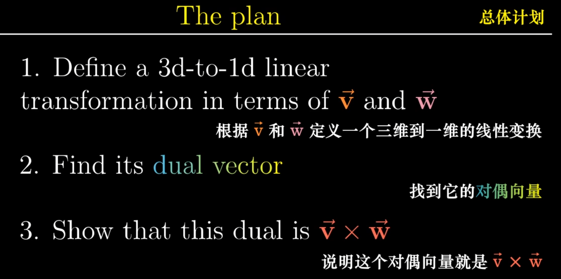
The cross product is deeply connected to the concept of duality. Taking the cross product with v and w can be defined via a 3D-to-1D linear transformation whose value is the determinant of the matrix formed by a variable vector (x, y, z) and the vectors v and w.

Chapter 9: Change of Basis

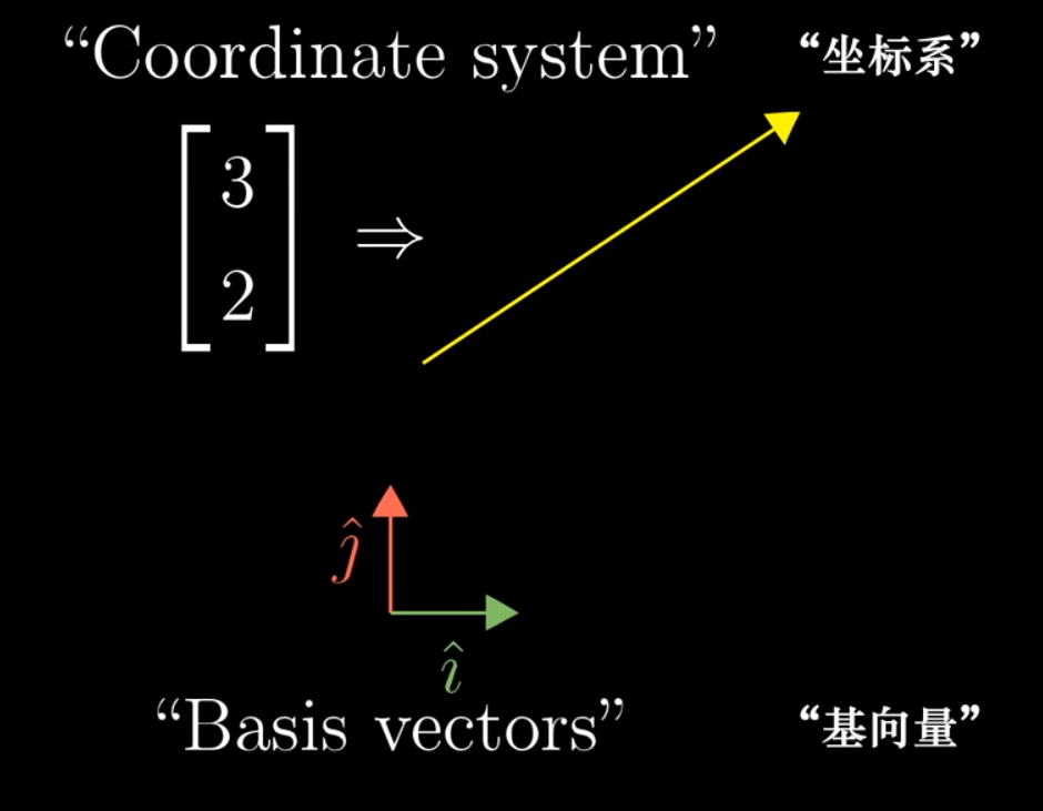
Any system that converts a vector into a set of coordinates is a coordinate system. This conversion is defined by the system’s basis vectors. Using a different set of basis vectors changes the mapping between vectors and their coordinates.

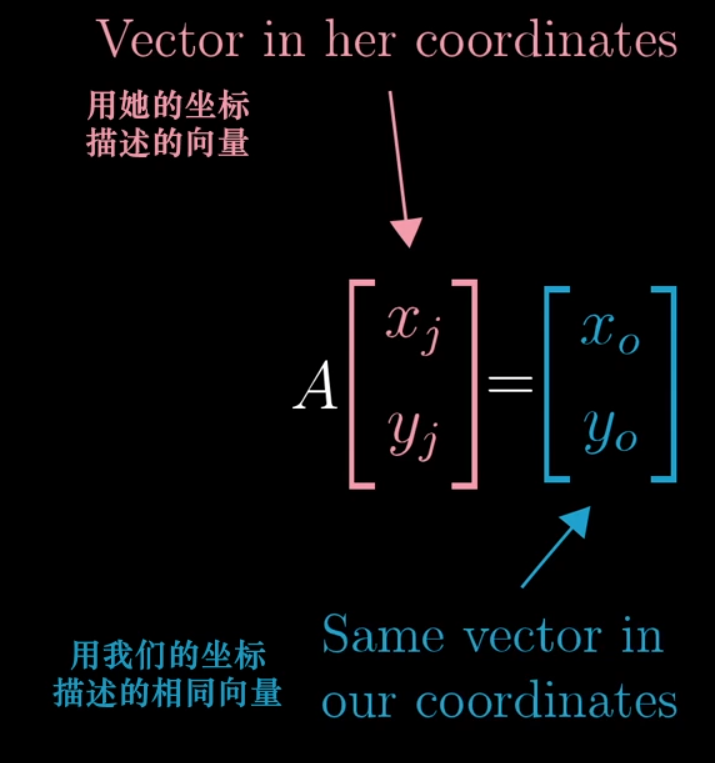
A change of basis matrix allows us to translate coordinates from one system to another.

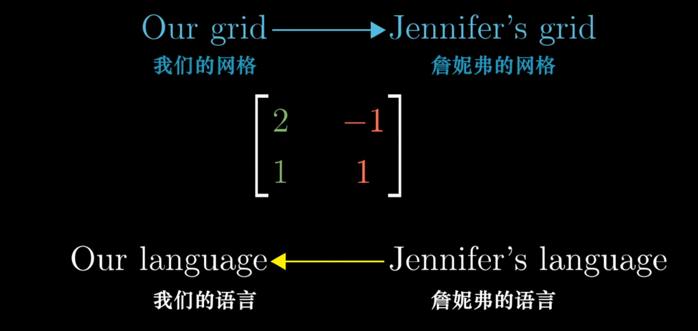
To translate a transformation matrix M from our standard coordinate system to an alternate basis, we use the formula P⁻¹MP, where P is the change of basis matrix for the alternate basis.

Chapter 10: Eigenvectors and Eigenvalues

Definition

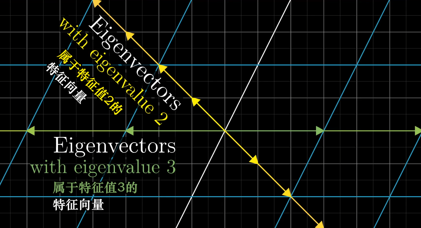
An eigenvector of a transformation is a non-zero vector that only gets scaled, not knocked off its original line, during the transformation.
An eigenvalue is the factor by which its corresponding eigenvector is scaled (stretched, compressed, or flipped).

Computational Idea

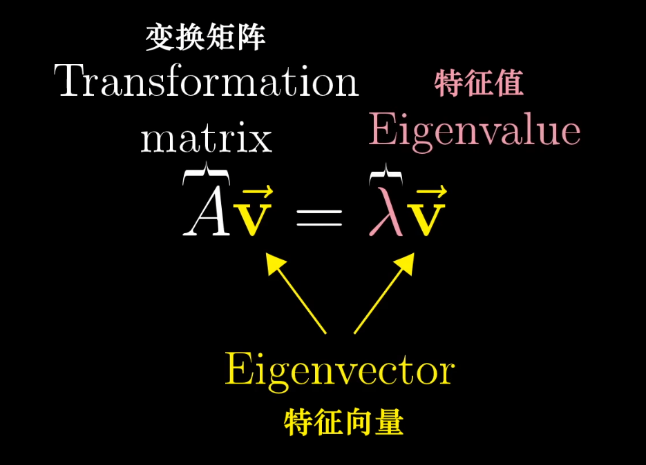
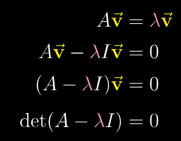
The defining equation is Av = λv, where A is the transformation matrix, v is an eigenvector, and λ is its eigenvalue. We can rearrange this to (A - λI)v = 0. For this equation to have a non-zero solution for v, the transformation (A - λI) must squish space into a lower dimension. This means its determinant must be zero.

So, we find eigenvalues by solving det(A - λI) = 0.

Eigenbasis

If we use eigenvectors as our basis vectors (an “eigenbasis”), calculations involving the transformation matrix become much simpler, as the matrix becomes diagonal with the eigenvalues on the diagonal.

Chapter 11: Abstract Vector Spaces

The Rigorous Definition of Linearity

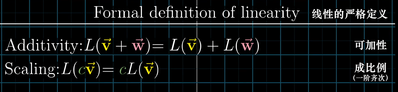
The property of linearity is what allows a linear transformation to be fully described by its action on the basis vectors, which is what makes matrix-vector multiplication possible.

(The derivative is a classic example of a linear operator.)

Functions as Vectors

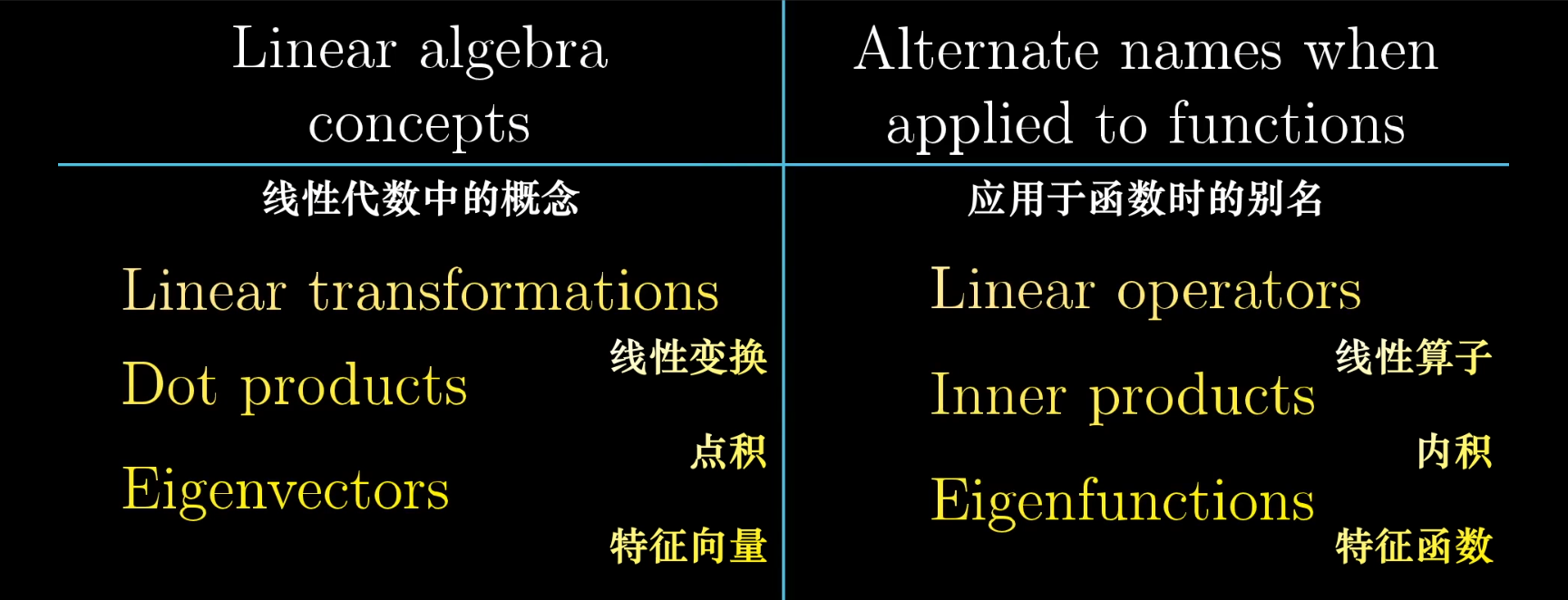
Vector Spaces

A vector space is an abstract concept. Anything that satisfies the fundamental axioms of vector addition and scalar multiplication can be considered a vector space, allowing us to apply the powerful tools of linear algebra.