「Algorithm4」2: Sorting

08 Oct 2023

Official Website: https://algs4.cs.princeton.edu/home/

Sorting

Sorting is the process of rearranging a collection of objects into a specific logical order. It holds significant importance in both business data processing and modern scientific computing. This chapter will focus on sorting algorithms, introducing, studying, and implementing several classic methods.

All sorting algorithms have been re-implemented in C++ and can be found in this GitHub repository.

Preliminaries

Utility Functions for Sorting Algorithms

Below are the definitions of some basic methods required for sorting. These functions provide a level of abstraction, allowing us to better track the algorithm’s execution process, such as the total number of comparisons and swaps.

void Swap(std::vector<int> &vec, int a, int b);
bool IsSmaller(const int &a, const int &b);
bool IsGreater(const int &a, const int &b);
bool IsEqual(const int &a, const int &b);
bool IsSorted(const std::vector<int> &vec);
bool IsSorted(const std::list<int> &list);
void PrintVec(const std::vector<int> &vec);
void PrintVec(const std::list<int> &list);

IsSmaller/IsGreater/IsEqual: Compare the values of two elements.
Swap: Swap two elements.
PrintVec: Print the contents of the array/list.
IsSorted: Check if the array/list is successfully sorted.

Bubble Sort

Bubble Sort works by repeatedly comparing and swapping adjacent elements. This process resembles bubbles rising from the bottom to the top, hence the name.

Implementation

void BubbleSort(std::vector<int> &vec) {
    const int size = static_cast<int>(vec.size());
    for (int i = size - 1; i > 0; --i)
        for (int j = 0; j < i; j++)
            if (IsGreater(vec[j], vec[j + 1]))
                Swap(vec, j, j + 1);
}

If a pass through the array (one “bubbling” phase) results in no swaps, it means the array is already sorted, and we can return immediately. Therefore, we can add a flag to detect this condition and optimize performance by exiting early.

void BubbleSortWithFlag(std::vector<int> &vec) {
    const int size = static_cast<int>(vec.size());
    for (int i = size - 1; i > 0; --i) {
        bool flag = false;
        for (int j = 0; j < i; j++)
            if (IsGreater(vec[j], vec[j + 1])) {
                Swap(vec, j, j + 1);
                flag = true;
            }
        if (!flag) break;
    }
}

Characteristics

Time Complexity: (O(n^2)), Adaptive: The lengths of the arrays traversed in each “bubbling” pass are (n-1, n-2, \dots, 2, 1), summing to ((n-1)n/2). With the flag optimization, the best-case time complexity can reach (O(n)).
Space Complexity: (O(1)), In-place: The pointers i and j use a constant amount of extra space.
Stable: It’s a stable sort because equal elements are never swapped.

Selection Sort

Selection Sort is one of the simplest sorting algorithms. Its core idea is to repeatedly select the minimum/maximum element.

We first find the minimum/maximum element in the array and swap it with the first element. Then, we find the minimum/maximum element among the remaining elements and swap it with the second element. This process is repeated until the last element.

Implementation

void SelectionSort(std::vector<int> &vec) {
    const int size = static_cast<int>(vec.size());
    for (int i = 0; i < size; i++) {
        int min_index = i;
        for (int j = i + 1; j < vec.size(); j++)
            if (IsSmaller(vec[j], vec[min_index]))
                min_index = j;
        if (min_index != i)
            Swap(vec, i, min_index);
    }
}

Analysis

For an array of length (N), Selection Sort requires approximately (N^2/2) comparisons and (N) swaps. Its time complexity is on the order of (N^2).

It has two distinct characteristics:

Runtime is independent of the input: The efficiency of Selection Sort is unaffected by the initial order of the array, whether it’s sorted or unsorted.
Minimal data movement: The number of swaps in Selection Sort is linear with the size of the array. No other sorting algorithm shares this feature (most are on the order of (N \log N) or (N^2)).

Characteristics

Time Complexity: (O(n^2)), Not Adaptive: The outer loop runs (n-1) times. The length of the unsorted section is (n) in the first round and 2 in the last, meaning the number of inner loop iterations is (n, n-1, \dots, 3, 2), summing to ((n-1)(n+2)/2).
Space Complexity: (O(1)), In-place: Pointers i and j use a constant amount of extra space.
Unstable: An element might be swapped to the right of another equal element, changing their relative order.

Insertion Sort

The core idea of Insertion Sort is like organizing a hand of playing cards: each new card is inserted into its proper place among the already sorted cards.

In the implementation, to make space for an element, we need to shift the other elements one position to the right. Similar to Selection Sort, the elements to the left of the current index are always sorted. When the index reaches the right end of the array, the sort is complete.

Implementation

void InsertionSort(std::vector<int> &vec) {
    const int size = static_cast<int>(vec.size());
    for (int i = 1; i < size; i++) {
        int num = vec[i], j = i;
        while (j > 0 && IsSmaller(num, vec[j - 1])) {
            vec[j] = vec[j - 1];
            j--;
        }
        vec[j] = num;
    }
}

Analysis

For an array of length (N), Insertion Sort’s time complexity is on the order of (N^2).

Insertion Sort is highly effective in certain situations. Its actual efficiency largely depends on the number of insertions it needs to perform.

An array is considered partially sorted if the number of inversions is less than a certain multiple of the array size. Here are some typical examples of partially sorted arrays:

Each element is not far from its final sorted position.
A large, sorted array is followed by a small, unsorted array.
Only a few elements are out of place.

Insertion Sort is very effective for such arrays, whereas Selection Sort is not. In fact, when the number of inversions is small, Insertion Sort is likely faster than any other algorithm.

Shell Sort

Shell Sort is an enhancement of Insertion Sort. Its core idea is to allow the exchange of far-apart elements to partially sort the array, and then use Insertion Sort to finalize the process.

As analyzed in the Insertion Sort section, it is very fast for partially sorted arrays. Shell Sort leverages this by first making the array partially sorted before applying a final sorting pass, thereby speeding up the process.

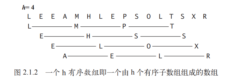
As shown below, Shell Sort divides the array into interleaved subarrays with a gap of h. For an array [5, 7, 1, 4, 6, 9] with (h=3), it would be split into three groups: [5, 4], [7, 6], and [1, 9]. Each group is sorted internally using Insertion Sort (or more simply, by swapping each element with larger elements preceding it in the subarray), resulting in [4, 5], [6, 7], and [1, 9]. This produces an h-sorted array. We then decrease h to create a more sorted array, eventually completing the sort.

From another perspective, a large h allows elements to move long distances, improving efficiency compared to Insertion Sort, where elements move one position at a time.

Our implementation below uses the sequence (1/2(3^k-1)), starting from (N/3) and decreasing to 1. This is known as an increment sequence. The implementation calculates this sequence on the fly; an alternative is to pre-store the sequence in an array.

Implementation

void ShellSort(std::vector<int> &vec) {
    const int size = static_cast<int>(vec.size());
    int h = size / 3;
    while (h >= 1) {
        for (int i = h; i < size; ++i) {
            int num = vec[i], j = i;
            while (j >= h && IsSmaller(num, vec[j - h])) {
                vec[j] = vec[j - h];
                j -= h;
            }
            vec[j] = num;
        }
        h /= 3;
    }
}

Analysis

Shell Sort is significantly faster than Insertion Sort.

The efficiency of Shell Sort comes from its trade-off between subarray size and sortedness.

Initially, the subarrays are short and are quickly sorted. After each pass, the array becomes more partially sorted, which are both conditions favorable for Insertion Sort.

The degree to which the array becomes partially sorted depends on the chosen increment sequence. Selecting the best sequence is a complex problem: the algorithm’s performance depends not only on the values of h but also on their mathematical properties, like their common factors. Many papers have studied various increment sequences, but none has been proven to be the “best”. Our implementation uses a simple, easily computed sequence, but more complex sequences have been proven to perform better. The discovery of even better increment sequences remains an open area of research.

A thorough understanding of Shell Sort’s performance is still a challenge. In fact, Shell Sort is the only sorting method for which we cannot accurately characterize its performance on a randomly ordered array.

Merge Sort

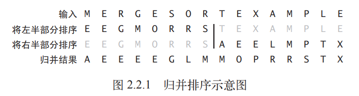
Merging is the process of combining two sorted arrays into a single, larger sorted array. Merge Sort is based on this simple operation.

Merge Sort is a recursive sorting algorithm based on the divide-and-conquer paradigm. To sort an array, it first recursively divides it into two halves, sorts each half, and then merges the results.

The main advantage of Merge Sort is its guarantee that sorting an array of length (N) takes time proportional to (N \log N). Its main disadvantage is that it requires extra space proportional to (N).

Abstract Merge Implementation

A straightforward way to implement the merge operation is to merge two separate sorted arrays into a third array. This involves creating an appropriately sized array and then copying elements from the two input arrays into it in sorted order.

void Merge(std::vector<int> &vec, const int left, const int mid, const int right) {
    const int length = right - left + 1;
    std::vector<int> temp(length);
    int i = left, j = mid + 1, k = 0;
    while (i <= mid && j <= right) {
        if (IsSmaller(vec[i], vec[j]))  temp[k++] = vec[i++];
        else                            temp[k++] = vec[j++];
    }
    while (i <= mid)    temp[k++] = vec[i++];
    while (j <= right)  temp[k++] = vec[j++];
    for (k = 0; k < length; ++k) {
        vec[k + left] = temp[k];
    }
}

The code above demonstrates a single merge operation, which requires creating a temporary auxiliary array.

While this code works for a single merge, sorting a large array requires many merges. The above method would copy the original array in its entirety for each merge, leading to significant memory consumption.

An “in-place merge” method that avoids using an extra array would be preferable, but implementing it is difficult and complex. Nevertheless, the above method is valuable as it provides a clear abstraction of the merge operation, which we can build upon.

Top-Down Merge Sort

Based on the abstract merge implementation, we can create a top-down, recursive merge sort algorithm. This is a classic example of applying the divide-and-conquer strategy in algorithm design.

Implementation

void MergeSortTopToBottom(std::vector<int> &vec, const int left, const int right) {
    if (left >= right) return;
    const int mid = (right + left) / 2;
    MergeSortTopToBottom(vec, left, mid);
    MergeSortTopToBottom(vec, mid + 1, right);
    Merge(vec, left, mid, right);
}

void MergeSortTopToBottom(std::vector<int> &vec) {
    const int size = static_cast<int>(vec.size());
    MergeSortTopToBottom(vec, 0, size - 1);
}

Analysis

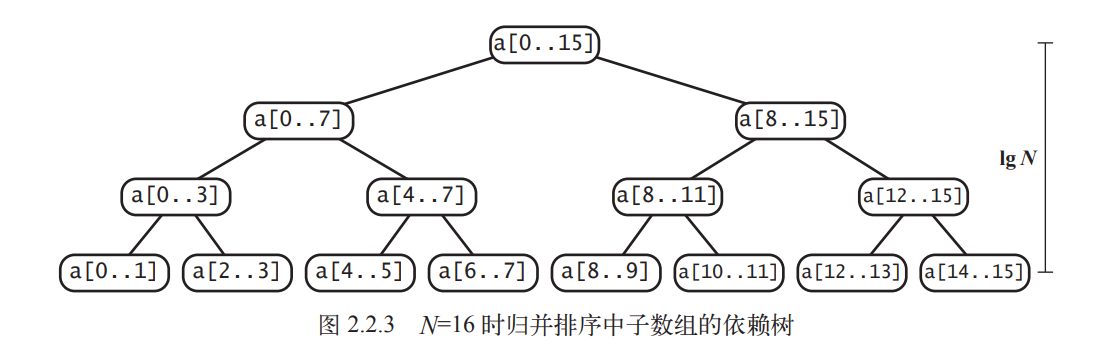
The image above shows the recursion tree for the top-down merge sort algorithm.

For any array of length N, top-down merge sort requires between (\frac{1}{2}N \log N) and (N \log N) comparisons and at most (6N \log N) array accesses.

Merge Sort is in a different league from the elementary sorting methods discussed earlier. It demonstrates that we can sort a massive array in a time that is only a logarithmic factor greater than the time needed to simply traverse it. Merge Sort can handle arrays of millions or even larger sizes, a feat impossible for Insertion Sort or Selection Sort.

Improvements

We can significantly improve the runtime of Merge Sort with a few careful modifications:

Use Insertion Sort for small subarrays: Recursion can lead to excessive method calls for small-scale problems. As we’ve seen, Insertion Sort can be faster than Merge Sort for small arrays. By switching to Insertion Sort when the array size is small enough, we can improve overall efficiency.
Test if the array is already sorted: We can add a check: if a[mid] is less than or equal to a[mid+1], the array is already sorted, and we can skip the merge() call. This change doesn’t affect the recursive calls but makes the algorithm’s runtime linear for any sorted subarray.
Avoid copying elements to the auxiliary array: We can save time by eliminating the copy to the auxiliary array used for merging. This technique requires switching the roles of the input and auxiliary arrays at each level of recursion. The merge process is like transcribing from a source text; this method alternates which array serves as the source.

The following code implements these three optimizations:

void MergeOptimized(const std::vector<int> &source, std::vector<int> &destination, const int left, const int mid, const int right) {
    int i = left, j = mid + 1, k = left;
    while (i <= mid && j <= right) {
        if (IsSmaller(source[i], source[j]))    destination[k++] = source[i++];
        else                                    destination[k++] = source[j++];
    }
    while (i <= mid)    destination[k++] = source[i++];
    while (j <= right)  destination[k++] = source[j++];
}

void MergeSortOptimized(std::vector<int> &source, std::vector<int> &destination, const int left, const int right) {
    static int kCUTOFF = 7;
    if (right - left <= kCUTOFF) {  // apply insertion sort for small subarrays
        InsertionSort(destination, left, right);
        return;
    }
    const int mid = (right + left) / 2;
    // *self-merge: avoid creating temp array when merging
    MergeSortOptimized(destination, source, left, mid);
    MergeSortOptimized(destination, source, mid + 1, right);
    // test if array is sorted before merge
    if (IsSmaller(source[mid], source[mid + 1])) {
        std::copy(source.begin() + left, source.begin() + right + 1, destination.begin() + left);
        return;
    }
    MergeOptimized(source, destination, left, mid, right);
}

void MergeSortOptimized(std::vector<int> &vec) {
    const int size = static_cast<int>(vec.size());
    std::vector aux_vec(vec);
    MergeSortOptimized(aux_vec, vec, 0, size - 1);
}

Bottom-Up Merge Sort

Recursive Merge Sort is a classic application of the divide-and-conquer strategy: we break a large problem into smaller ones, solve them individually, and then combine their solutions to solve the original problem. Although we think of merging two large arrays, in practice, most of the merged arrays are very small.

In top-down Merge Sort, we start with the large array and progressively divide it. We can also start directly with the small arrays. Imagine each element as a sorted array of size 1. We can then merge them in pairs, then in fours, then eights, and so on, until the entire array is sorted. This implementation of Merge Sort is called Bottom-Up Merge Sort.

Implementation

void MergeSortBottomToTop(std::vector<int> &vec) {
    const int size = static_cast<int>(vec.size());
    for (int length = 1; length < size; length *= 2) {
        for (int left = 0; left < size - length; left += 2 * length) {
            const int mid = left + length - 1;
            const int right = std::min(left + 2 * length - 1, size - 1);
            Merge(vec, left, mid, right);
        }
    }
}

Analysis

For any array of length (N), bottom-up merge sort requires between (\frac{1}{2}N \log N) and (N \log N) comparisons, and at most (6N \log N) array accesses.

An advantage of this implementation is that it requires less code than the standard recursive approach.

When the array length is a power of 2, top-down and bottom-up merge sorts perform the exact same number of comparisons and array accesses, just in a different order. For other lengths, the sequence of comparisons and accesses will differ.

Bottom-up Merge Sort is particularly well-suited for data organized in a linked list, as it can sort the list in-place by reorganizing links without creating any new nodes.

It is natural to implement any divide-and-conquer algorithm using either a top-down or a bottom-up approach.

Complexity of Sorting Algorithms

Studying Merge Sort is important because it forms the basis for a significant conclusion in the field of computational complexity.

For comparison-based sorting algorithms, the following property holds (here, we ignore the overhead of array accesses):

No comparison-based algorithm can guarantee sorting an array of length (N) with fewer than (\log(N!) \sim N \log N) comparisons.

The book provides an elegant proof of this conclusion using a binary tree-based mathematical model, which will not be detailed here.

This property establishes an upper bound and a target for sorting algorithm design. Without this conclusion, we might waste effort trying to design a comparison-based algorithm with, say, half the number of worst-case comparisons as Merge Sort. This conclusion tells us that such an algorithm does not exist.

In our analysis of Merge Sort, we found its worst-case number of comparisons to be (N \log N). Since no sorting algorithm can do better than (\log(N!) \sim N \log N) comparisons, this means:

Merge Sort is an asymptotically optimal comparison-based sorting algorithm.

Strictly speaking, an algorithm is only optimal if it requires exactly (\log N!) comparisons. In practice, however, the difference between such an algorithm and Merge Sort is negligible, even for very large (N).

Although we’ve established that Merge Sort is asymptotically optimal, it still has limitations:

Its space complexity is not optimal.
Worst-case scenarios may not be encountered in practice.
Other operations besides comparisons (e.g., array accesses) can also be important.
Some data can be sorted without comparisons.

Quick Sort

Finally, we arrive at the renowned Quick Sort, arguably the most widely used sorting algorithm. It is simple to implement, has low dependency on the input, and is generally much faster than other sorting algorithms in typical applications. It is excellent in terms of both memory and efficiency.

Memory: Quick Sort is an in-place algorithm, requiring only a small auxiliary stack.
Efficiency: The time required to sort an array of length (N) is proportional to (N \log N).

Basic Implementation

Like Merge Sort, Quick Sort is a recursive, divide-and-conquer algorithm. Both divide the array and sort the pieces separately, but their approaches are philosophically opposite, or complementary:

Merge Sort divides the array, sorts the resulting subarrays, and then merges the sorted subarrays to sort the entire array. In essence, Merge Sort is “recurse first, process later.”
Quick Sort partitions the array based on element values, such that when both subarrays are sorted, the entire array is naturally sorted. It is “process first, recurse later.”

Figuratively, Merge Sort completes the sorting on its way back up the recursion tree, while for Quick Sort, the sorting is already complete when it reaches the base case.

Correspondingly, Merge Sort uses a recursive merge operation to sort, while Quick Sort uses a partition operation.

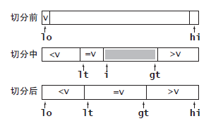
When partitioning an array, we select a “pivot” element. Then, through swaps, we rearrange the array so that all elements to the left of the pivot are smaller than it, and all elements to its right are larger.

By recursively partitioning the array, we can sort it. This is the fundamental principle of Quick Sort.

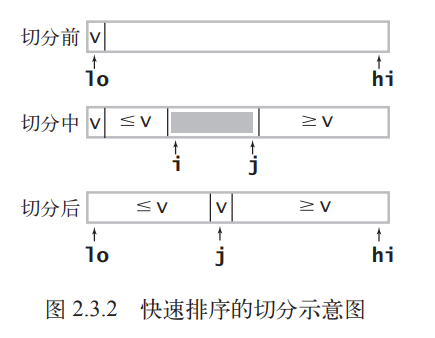
As shown above, a common strategy for partitioning is to pick an arbitrary element as the pivot—here, we’ll use a[lo], the leftmost element. We then use a pointer i to scan from the left until we find an element greater than or equal to the pivot, and another pointer j to scan from the right until we find an element less than or equal to it. These two elements are clearly out of place, so we swap them. We continue this process until i and j cross, at which point we swap the pivot element into its final position.

Here is a basic implementation of Quick Sort:

int Partition(std::vector<int> &vec, const int left, const int right) {
    const int item = vec[left];
    int i = left, j = right + 1;
    while (true) {
        // stop even if vec[i/j] == item; this may cause extra swaps, but it can optimize element distribution
        while (IsSmaller(vec[++i], item)) if (i == right) break; // prevent out-of-bounds
        while (IsGreater(vec[--j], item)) if (j == left) break;
        if (i >= j) break;
        Swap(vec, i, j);
    }
    Swap(vec, left, j);
    return j;
}

void QuickSort(std::vector<int> &vec, const int left, const int right) {
    if (left >= right) return;
    const int mid = Partition(vec, left, right);
    QuickSort(vec, left, mid - 1);
    QuickSort(vec, mid + 1, right);
}

void QuickSort(std::vector<int> &vec) {
    const int size = static_cast<int>(vec.size());
    QuickSort(vec, 0, size - 1);
}

Avoiding Pitfalls

Quick Sort has numerous advantages, but it is also “fragile.” A poor implementation can easily lead to terrible performance, turning Quick Sort into “Slow Sort” 🤣.

Here are some key points:

In-place partitioning: We could easily implement partitioning with an auxiliary array like in Merge Sort, but the associated memory and efficiency costs would be self-defeating.
Array out-of-bounds issues: In the inner loops of partitioning, we scan the array based on the pivot. If the pivot is the smallest or largest element, an out-of-bounds access can occur. In our implementation, if (i == right) break and if (j == left) break prevent this. However, the if (j == left) break is redundant because our pivot is the leftmost element, and vec[j] will never be smaller than vec[left]. This check can be removed. In this case, the pivot itself acts as a “sentinel.” We could also manually place a sentinel (the largest element) at the rightmost end of the array, which would eliminate the need for if (i == right) break as well.
Shuffle the array to maintain randomness: Shuffling the array before sorting ensures the reliability of performance tests. It also prevents Quick Sort from exhibiting worst-case (O(N^2)) performance on certain inputs, such as when the pivot is always the smallest or largest element.
Loop termination conditions: Correctly checking for pointer bounds requires some care. A common mistake is failing to account for elements equal to the pivot.
Handling duplicate keys: The left scan should stop on elements greater than or equal to the pivot, and the right scan on elements less than or equal to the pivot. While this might cause unnecessary swaps of equal elements, it prevents the runtime from degrading to quadratic in certain common cases. We will later discuss a better way to handle arrays with many duplicates.
Recursion termination condition: A common mistake is failing to place the pivot correctly, which can lead to infinite recursion if the pivot is the smallest or largest element in a subarray.

Analysis

A key reason for Quick Sort’s high efficiency is its simple and fast partitioning inner loop. The partitioning method compares array elements with a fixed value using an incrementing index, whereas Shell Sort and Merge Sort involve data movement within their inner loops.

Another speed advantage of Quick Sort is its low number of comparisons.

To sort an array of N distinct elements, Quick Sort requires, on average, (\sim 2N \ln N) comparisons (and (\frac{1}{6}) of that in swaps).

In summary, the runtime of Quick Sort for an array of size (N) is within a constant factor of (1.39N \lg N). Merge Sort also achieves this, but Quick Sort is generally faster (despite making 39% more comparisons) because it moves less data. These guarantees are derived from probability theory.

Improvements

Quick Sort was invented by C.A.R. Hoare in 1960, and since then, numerous improvements have been proposed. Not all ideas are practical, as Quick Sort is already well-balanced, and improvements can be offset by unintended side effects. However, some, which we will introduce now, are very effective.

Use Insertion Sort for small subarrays

We used this same technique to improve Merge Sort, and the idea here is similar.

For small arrays, Quick Sort is slower than Insertion Sort.
Due to recursion, Quick Sort’s QuickSort() method is called frequently on small arrays.

void QuickSort(std::vector<int> &vec, const int left, const int right) {
    static int kCUTOFF = 7;
    if (right - left <= kCUTOFF) { // apply insertion sort for small subarrays
        InsertionSort(vec, left, right);
        return;
    }
    const int mid = Partition3Sample(vec, left, right);
    QuickSort(vec, left, mid - 1);
    QuickSort(vec, mid + 1, right);
}

The optimal value for the cutoff threshold kCUTOFF is system-dependent, but any value between 5 and 15 is generally satisfactory.

Median-of-three partitioning

Quick Sort’s efficiency largely depends on the choice of the pivot. The optimal case is when the pivot is the median of the array elements. However, calculating the true median would require a full scan at each partitioning step, which is not cost-effective.

In our current implementation, we shuffle the array to eliminate input dependency, making the pivot selection random and achieving average performance without calculating the median.

An alternative is median-of-three partitioning, which uses the median of a small sample of elements from the subarray as the pivot. This leads to better partitions. While it incurs the cost of finding a median, it’s much cheaper than scanning the whole subarray. A sample size of 3 has been found to work best in practice.

An added benefit of this method is that the sample elements can serve as sentinels, eliminating the need for boundary checks in the partitioning loop.

int Partition3Sample(std::vector<int> &vec, const int left, const int right) {
    // sample item at left/mid/right
    const int mid = (left + right) / 2;
    if (IsGreater(vec[mid], vec[right])) Swap(vec, right, mid);
    if (IsGreater(vec[mid], vec[left])) Swap(vec, left, mid);
    if (IsGreater(vec[left], vec[right])) Swap(vec, left, right);
    const int item = vec[left];
    int i = left, j = right + 1;
    while (true) {
        while (IsSmaller(vec[++i], item)) {} // sentinel at right prevents out-of-bounds
        while (IsGreater(vec[--j], item)) {} // sentinel at left prevents out-of-bounds
        if (i >= j) break;
        Swap(vec, i, j);
    }
    Swap(vec, left, j);
    return j;
}

Entropy-Optimal Sorting - 3-Way Partitioning

In real-world applications, sorting algorithms often encounter inputs with many duplicate keys, such as sorting by birthday or gender. In these cases, Quick Sort’s performance can be significantly improved. For example, on an array of all equal elements, the standard Quick Sort will still partition it.

A solution to this problem is 3-way partitioning, which divides the array into three parts: elements smaller than the pivot, elements equal to the pivot, and elements greater than the pivot. This is more complex to design, but Dijkstra proposed a concise implementation that uses an additional pointer to manage the “equal to” section.

void QuickSort3Way(std::vector<int> &vec, const int left, const int right) {
    if (left >= right) return;
    int less_then_i = left, i = left + 1, greater_than_i = right;
    const int item = vec[left];
    while (i <= greater_than_i) {
        if (IsSmaller(vec[i], item)) {
            Swap(vec, less_then_i++, i++);
        } else if (IsGreater(vec[i], item)) {
            Swap(vec, greater_than_i--, i);
        } else {
            i++;
        }
    }
    QuickSort3Way(vec, left, less_then_i - 1);
    QuickSort3Way(vec, greater_than_i + 1 , right);
}

Priority Queues (Heap Sort)

In some practical applications of sorting, we don’t always need the entire dataset to be globally ordered. For instance, when scheduling application priorities, we only need to ensure that the highest-priority task is always processed first. A Priority Queue is an abstract data type designed for this purpose, typically supporting two main operations: delete the maximum element and insert an element.

Elementary PQ Implementations

We can quickly implement a priority queue using previous sorting algorithms like Insertion Sort. We could simply call a sorting algorithm whenever an element is accessed or inserted. This approach is essentially a wrapper around a sorting algorithm and offers limited improvement in speed or memory usage.

Binary Heap-Based Priority Queue

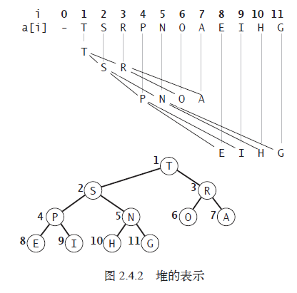
A binary heap is a complete binary tree where each node is greater than or equal to its two children.

A binary heap is an excellent data structure for implementing a priority queue. Due to its properties, we can represent a binary heap using an array. For a node at index (k), its children are at indices (2k) and (2k+1), and its parent is at index (k/2).

class MaxPriorityQueue {
public:
    MaxPriorityQueue() { pq_.push_back(0); }

    void Insert(int key) {
        pq_.push_back(key);
        Swim(static_cast<int>(pq_.size()) - 1);
    }

    int ExtractMax() {
        if (pq_.size() <= 1) throw std::runtime_error("queue is empty");
        int max = pq_[1];
        pq_[1] = pq_.back();
        pq_.pop_back();
        Sink(1);
        return max;
    }

    [[nodiscard]] int GetMax() const {
        if (pq_.size() <= 1) throw std::runtime_error("queue is empty");
        return pq_[1];
    }
    [[nodiscard]] bool IsEmpty() const { return pq_.size() <= 1; }
    [[nodiscard]] size_t GetSize() const { return pq_.size() - 1; }
private:
    std::vector<int> pq_;

    void Swim(int i) {
        while (i > 1 && pq_[i / 2] < pq_[i]) {
            Swap(pq_, i / 2, i);
            i /= 2;
        }
    }

    void Sink(int i) {
        int child = 2 * i;
        while (child < pq_.size()) {
            if (child < pq_.size() - 1 && pq_[child] < pq_[child + 1]) child++;
            if (pq_[i] >= pq_[child]) break;
            Swap(pq_, i, child);
            i = child;
            child = 2 * i;
        }
    }
};

The code above is a basic implementation of a max-heap in C++. It uses std::vector as the underlying container, and we skip index 0 of the array to simplify the parent-child index relationship.

Two operations are crucial for implementing a binary heap:

Swim: Bottom-up heap reordering. When an element is inserted, it may be larger than its parent. We need to “swim” it up by repeatedly swapping it with its parent until it reaches the root or is smaller than its parent.
Sink: Top-down heap reordering. When the maximum element is deleted, we replace the root with another element from the heap (in this implementation, the last one). This may violate the heap property, so we need to “sink” the new root down by repeatedly swapping it with its larger child.

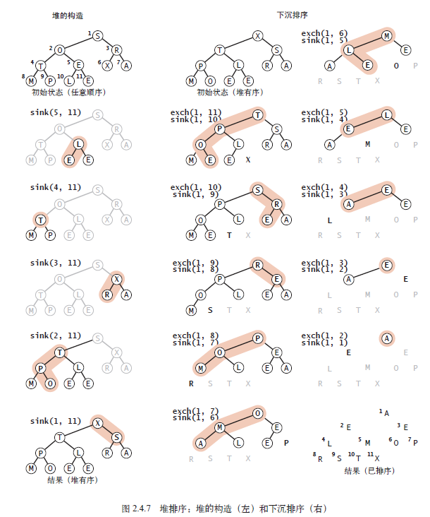
Heap Sort

We can adapt the priority queue into a sorting algorithm called Heap Sort, which consists of two phases:

Heap Construction: Rearrange the initial data into a heap.
Sortdown: Sequentially extract all elements from the heap to get the final sorted result.

The simplest implementation of Heap Sort is to construct a new heap, insert every element from the array to be sorted, and then extract the maximum/minimum elements one by one.

void HeapSort(std::vector<int> &vec) {
    MaxPriorityQueue pq;
    for (int i : vec) pq.Insert(i);
    for (int &i : vec) i = pq.ExtractMax();
}

Implementing Heap Sort this way creates a new heap, resulting in (O(N)) space complexity. However, we can perform the sort in-place.

Furthermore, constructing the heap using the Insert method requires (N) calls to Swim. A more clever approach is to use the Sink function for heap construction. We can view the array as a collection of small heaps. By calling Sink on the root of each small heap, we can merge them. If a node’s two children are already roots of heaps, calling Sink on that node will merge them into a larger heap. This allows for recursive heap construction.

The advantage of this approach is that we can skip the elements at the bottom level of the heap since they have no children. This reduces the number of Sink calls to (N/2), half of what the Insert-based method requires.

void SinkFrom0(std::vector<int> &vec, int root, int end) {
    int child = 2 * root + 1;
    while (child <= end) {
        if (child < end && IsSmaller(vec[child], vec[child + 1])) child++;
        if (IsGreater(vec[root], vec[child]) || IsEqual(vec[root], vec[child])) break;
        Swap(vec, root, child);
        root = child;
        child = 2 * root + 1;
    }
}

void HeapSortInPlace(std::vector<int> &vec) {
    const int size = static_cast<int>(vec.size());
    for (int i = size / 2 - 1; i >= 0; i--) SinkFrom0(vec, i, size - 1);
    for (int i = size - 1; i > 0; i--) {
        Swap(vec, 0, i);
        SinkFrom0(vec, 0, i - 1);
    }
}

Heap Sort holds an important place in the study of sorting complexity. It is the only known method that is optimal in both space and time usage—it guarantees (～2N \lg N) comparisons in the worst case with constant extra space. Heap Sort is popular when space is at a premium (e.g., in embedded systems or low-cost mobile devices) because it achieves good performance with just a few lines of code (even in machine code).

However, it is rarely used in many modern systems because it cannot take advantage of caching. Array elements are rarely compared with adjacent elements, leading to a much higher number of cache misses than algorithms where most comparisons are between neighbors, such as Quick Sort, Merge Sort, and even Shell Sort.

Summary and Addendum

Stability of Sorting Algorithms

A sorting algorithm is considered stable if it preserves the relative order of equal elements in the array.

While stability is a desirable property, and there are ways to make any sorting algorithm stable, stable sorts are generally advantageous only when stability is a strict requirement. In fact, no common method achieves stability without using a significant amount of extra time and space.

Comparison of Sorting Algorithms

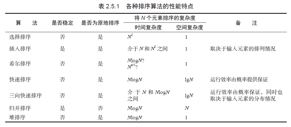
In most practical situations, Quick Sort is the best choice. It is the fastest general-purpose sorting algorithm.