「Algorithm4」1: Fundamentals
13 Sep 2023
Official Website: https://algs4.cs.princeton.edu/home/
Basic Programming Model
Algorithms, 4th Edition primarily uses Java as its programming language. This section provides an overview of Java’s fundamentals.
Java Basics
Compilation Process
Java is a language designed entirely around the principles of Object-Oriented Programming (OOP), where all code is organized within class structures.
In Java, we write source code in files with a .java extension. Each .java file typically contains a public class with the same name as the file. Any class can contain a main method, which serves as the program’s entry point.
The javac command in the command line compiles a .java file, producing a .class file containing Java bytecode. The java command then executes the main method within this .class file.
How Java Works
Java is a hybrid language that is both compiled and interpreted. It first compiles high-level source code into platform-independent Java bytecode, which is then executed by the Java Virtual Machine (JVM).
This architecture grants Java excellent cross-platform compatibility. As long as a platform has a corresponding JVM implementation, it can run any Java bytecode.
Furthermore, the JVM performs run-time optimizations, allowing Java to achieve speeds faster than purely interpreted languages. This process also enables certain run-time features of the language.
Redirection, Pipes, and I/O
Standard Input
In Java, the main method accepts a String[] args parameter, which receives command-line arguments.
When we run a .class file using the java command (without the file extension), we can pass arguments directly after the class name.
java Test abc 123 qwe
In the command above, we execute Test.class. The subsequent arguments abc, 123, and qwe are passed into the program as String[] args = {"abc", "123", "qwe"};.
Standard Output
Typically, we can use the standard System.out library or the book’s custom StdOut library to print content to the console.
The StdOut library also supports formatted output, similar to printf() in C/C++. Its usage is straightforward and not detailed further here.
Redirection
Standard input and output involve interaction with the console, which can be inconvenient for handling large amounts of data.
Redirection allows us to read input directly from a text file or write output to a file. The input redirection operator is <, and the output operator is >.
java Test < data.txt > output.txt
This command instructs the program to read its input from data.txt and write its output to output.txt.
Redirected input can also be used in conjunction with standard command-line arguments.
java Test data1.txt < data2.txt
In this case, String[] args will contain {"data1.txt", ...}, where ... represents the content read from data2.txt.
Pipes
Pipes extend the concept of redirection by allowing the output of one program to become the input of another. The pipe operator is |.
java Test1 100 200 | java Test2
This command runs Test1.class with args = {"100", "200"}, and then pipes the output of Test1 as the input to Test2.class.
Data Abstraction
A data type is a set of values and a collection of operations on those values. This section covers the definition and use of data types, a process known as data abstraction.
Using Abstract Data Types (ADTs)
APIs and Inheritance
We use an Application Programming Interface (API) to describe the functions and methods of an abstract data type. This is similar to a library of static methods.
We can also extend classes and override methods from the parent class to flexibly adapt the API.
Objects
Unlike static method libraries, data types are typically instantiated as objects.
An object is an entity that holds a value of a data type.
All objects have three key characteristics:
- State: The value held by the data type.
- Identity: A reference to the object’s location in memory.
- Behavior: The operations that can be performed on the data type.
The sole responsibility of a data type’s implementation is to maintain an object’s identity. This allows client code to use the data type by adhering to the API that describes its behavior, without needing to know how its state is represented internally.
Creating Objects
Values of a data type are stored in objects, which are created (or instantiated) using the new keyword.
Counter heads = new Counter("Header");
When we use new, the system performs the following steps:
- Allocates memory for the new object.
- Calls the constructor to initialize the object.
- Returns a reference to the object.
We can create countless objects from the same class.
Object Assignment
When assigning a reference-type variable to another, we are essentially creating an alias by copying the memory address. This is a shallow copy, a point to be mindful of during use.
Summary of Objects
Writing code using the principles of data abstraction is known as Object-Oriented Programming (OOP), a critically important programming paradigm.
An implementation of a data type supports the following operations:
- Create objects: Use
newto invoke a constructor, which creates and initializes an object and returns a reference to it. - Operate on object values: Call instance methods using the variable associated with the object to manipulate its values.
- Work with multiple objects: Create arrays of objects and pass them to or return them from methods just like primitive data types. The key difference is that variables hold references to objects, not the objects themselves.
Implementing Abstract Data Types
The Counter Class
public class Counter
{
    // Instance variables
    private final String name; // `final` is similar to `const` in C#
    private int count;

    // Constructor
    public Counter(String id)
    {
        name = id;
    }

    // Instance methods
    public void increment()
    {
        count++;
    }

    public int tally()
    {
        return count;
    }

    public String toString()
    {
        return count + " " + name;
    }

    // Test client
    public static void main(String[] args)
    {
        Counter heads = new Counter("Heads");
        Counter tails = new Counter("Tails");

        heads.increment();
        heads.increment();
        tails.increment();

        StdOut.println(heads + " " + tails);
        StdOut.println(heads.tally() + tails.tally());
    }
}
The VisualAccumulator Class
public class VisualAccumulator
{
    private double total;
    private int n;

    public VisualAccumulator(int trials, double max)
    {
        StdDraw.setXscale(0, trials);
        StdDraw.setYscale(0, max);
        StdDraw.setPenRadius(.005);
    }

    public void addDataValue(double value)
    {
        n++;
        total += value;
        StdDraw.setPenColor(StdDraw.DARK_GRAY);
        StdDraw.point(n, value);
        StdDraw.setPenColor(StdDraw.RED);
        StdDraw.point(n, total / n);
    }

    public double mean()
    {
        return total / n;
    }

    public String toString()
    {
        return "Mean (" + n + " values): " + String.format("%7.5f", mean());
    }

    public static void main(String[] args)
    {
        int T = Integer.parseInt(args[0]);
        VisualAccumulator visualAccumulator = new VisualAccumulator(T, 1.0);
        for (int i = 0; i < T; i++)
            visualAccumulator.addDataValue(StdRandom.uniformDouble());
        StdOut.println(visualAccumulator);
    }
}
Designing Data Types
An abstract data type is a data type whose internal representation is hidden from the client.
Encapsulation
A key feature of OOP is encapsulation, where the implementation of a data type encapsulates its data. This simplifies the implementation and isolates it from client code development.
Encapsulation enables modular programming, allowing us to:
- Develop client and implementation code independently.
- Switch to an improved implementation without affecting client code.
- Support programs that have not yet been written.
Encapsulation also isolates the data type’s operations, which helps to:
- Limit the scope of potential errors.
- Add debugging tools like consistency checks within the implementation.
- Ensure client code is clearer and more maintainable.
Encapsulation is crucial for achieving high scalability. The key to successful modular programming is maintaining independence between modules.
Designing APIs
Designing a good API is one of the most important and challenging tasks in modern software development. There is no single correct answer; it requires experience, careful thought, and iterative refinement.
This motto may be helpful: Provide clients with the functionality they need, and nothing more.
Algorithms and ADTs
Data abstraction is a natural fit for the study of algorithms. It allows us to:
- Precisely define what an algorithm can provide to a client.
- Isolate the algorithm’s implementation from the client code.
- Build multiple layers of abstraction, implementing new algorithms using existing ones.
Equivalence
When we test for equivalence between reference types, such as a == b, we are comparing their references (i.e., their identities).
To compare their states, we can implement the equals() method from the Object class.
Java conventions require that equals() must implement an equivalence relation, which has the following properties:
- Reflexive:
x.equals(x)istrue. - Symmetric: If
x.equals(y)istrue, theny.equals(x)must betrue. - Transitive: If
x.equals(y)andy.equals(z)are bothtrue, thenx.equals(z)must betrue. - Consistent: Repeated calls to
x.equals(y)return the same result, provided the objects are not modified. - Non-null:
x.equals(null)is alwaysfalse.
Immutability
We can mark a variable as immutable using the final keyword, which means its value cannot be changed after its initial assignment.
It’s important to note that for reference types, final only guarantees the immutability of the reference itself (i.e., the variable will always point to the same memory location). It does not guarantee that the content at that memory location will remain unchanged.
Exceptions and Assertions
- Exceptions are typically used to handle unforeseen errors that are beyond our control.
- Assertions are used to verify assumptions we make in our code.
An assertion is a boolean expression. If the expression evaluates to false at runtime, the program will throw an error. Assertions are useful during testing to validate our logic and aid in debugging, ensuring that the code doesn’t terminate due to system errors or enter infinite loops. However, they should not be relied upon in production code, as they may be disabled.
Design by Contract: Data type designers should specify preconditions (conditions the client must satisfy before calling a method), postconditions (requirements the implementation must meet upon returning), and side effects (any other changes the method might make to the object’s state).
Bags, Queues, and Stacks
This section introduces three fundamental data types: the Bag, the Queue, and the Stack.
APIs
public class Bag<T> implements Iterable<T>
{
    Bag();              // Create an empty bag
    void add(T item);   // Add an item
    boolean isEmpty();  // Is the bag empty?
    int size();         // Number of items in the bag
}

public class Queue<T> implements Iterable<T>
{
    Queue();            // Create an empty queue
    void enqueue(T item); // Add an item
    T dequeue();        // Remove the least recently added item
    boolean isEmpty();    // Is the queue empty?
    int size();           // Number of items in the queue
}

public class Stack<T> implements Iterable<T>
{
    Stack();            // Create an empty stack
    void push(T item);  // Add an item
    T pop();            // Remove the most recently added item
    boolean isEmpty();  // Is the stack empty?
    int size();         // Number of items in the stack
}
Generics
Generics, also known as parameterized types, allow us to store data of any type.
We can replace the type parameter <T> with any reference type.
Stack<String> stack = new Stack<String>();
Autoboxing
Type parameters must be instantiated with reference types. Java has a special mechanism called autoboxing that enables generic code to work with primitive types.
Each primitive type in Java has a corresponding wrapper class (e.g., Integer for int, Boolean for boolean). Java automatically converts between them.
The automatic conversion of a primitive type to its wrapper type is called autoboxing. The reverse process is called unboxing.
Bags
A bag is a collection data type that does not support removing specific items. Its purpose is to help clients collect items and iterate through them.
The order of iteration in a bag is not specified. While a stack or queue could also be used for this purpose, using a bag explicitly indicates that the processing order of elements is not important.
Below is a program that uses a Bag to calculate the mean and standard deviation of a set of numbers.
public class Stats
{
    public static void main(String[] args)
    {
        Bag<Double> numbers = new Bag<Double>();

        while (!StdIn.isEmpty())
            numbers.add(StdIn.readDouble());

        int N = numbers.size();

        double sum = 0.0;
        for (double x : numbers)
            sum += x;
        double mean = sum / N;

        sum = 0.0;
        for (double x : numbers)
            sum += (x - mean) * (x - mean);
        double std = Math.sqrt(sum / (N - 1));

        StdOut.printf("Mean: %.2f\n", mean);
        StdOut.printf("Std dev: %.2f\n", std);
    }
}

/*
Input/Output:
100
101
98
65
^D
Mean: 91.00
Std dev: 17.38
*/
FIFO Queues
A queue is a collection type based on a first-in, first-out (FIFO) policy.
This is a common data structure in C++, C#, and other languages, so it is not discussed in further detail here.
Queue<Integer> queue = new Queue<Integer>();
When iterating through a queue using a foreach loop, elements are processed in the order they were added.
Pushdown Stacks
A stack is a collection type based on a last-in, first-out (LIFO) policy.
This is also a common data structure and is not discussed in further detail here.
Stack<Integer> stack = new Stack<Integer>();
When iterating through a stack using a foreach loop, elements are processed in the reverse order of their addition.
Arithmetic Expression Evaluation
We can evaluate arithmetic expressions in string format using Dijkstra’s two-stack algorithm.
An expression consists of parentheses, operators, and operands. We process these entities from left to right according to four cases:
- Push operands onto the operand stack.
- Push operators onto the operator stack.
- Ignore left parentheses.
- Upon encountering a right parenthesis, pop an operator, pop the required number of operands, and push the result of the operation onto the operand stack.
The final value remaining on the operand stack is the result of the expression. Here is the Java implementation:
public class Evaluate
{
    public static void main(String[] args)
    {
        // Dijkstra's two-stack algorithm for arithmetic expression evaluation
        Stack<String> operators = new Stack<>();
        Stack<Double> values = new Stack<>();
        while (!StdIn.isEmpty())
        {
            // Read token
            String s = StdIn.readString();
            if (s.equals("("))
                continue; // Ignore left parenthesis
            else if (s.equals("+") || s.equals("-") || s.equals("*") || s.equals("/") || s.equals("sqrt"))
            {
                operators.push(s); // Push operator
            }
            else if (s.equals(")"))
            {
                // Pop operator and operands, push result
                String operator = operators.pop();
                Double value = values.pop();
                if (operator.equals("+"))
                    values.push(values.pop() + value);
                else if (operator.equals("-"))
                    values.push(values.pop() - value);
                else if (operator.equals("*"))
                    values.push(values.pop() * value);
                else if (operator.equals("/"))
                    values.push(values.pop() / value);
                else if (operator.equals("sqrt"))
                    values.push(Math.sqrt(value));
            }
            else
            {
                // Push operand
                values.push(Double.parseDouble(s));
            }
        }
        StdOut.println(values.pop());
    }
}

/*
Input/Output:
( ( 1 + sqrt ( 5.0 ) ) / 2.0 )
^D
1.618033988749895
*/
This code is effectively a very simple “interpreter.”
Implementing Collection Data Types
Now, let’s implement these data structures ourselves.
Fixed-Capacity Stack
We’ll start with the simplest implementation: a fixed-capacity stack for strings. It requires the client to specify a capacity and does not support iteration.
public class FixedCapacityStackOfStrings
{
    private String[] s;
    private int N;

    public FixedCapacityStackOfStrings(int capacity)
    { s = new String[capacity]; }

    public boolean isEmpty()
    { return N == 0; }

    public int size()
    { return N; }

    public void push(String item)
    { s[N++] = item; }

    public String pop()
    { return s[--N]; }
}
This is a very basic data structure, but it forms the foundation for more complex ones.
Generics
The first limitation of our stack is that it can only handle String types. Generics solve this problem.
Note that due to legacy reasons, Java does not allow the direct creation of generic arrays. We can work around this by casting: T[] s = (T[]) new Object[capacity];.
public class FixedCapacityStack<T>
{
    private T[] s;
    private int N;

    public FixedCapacityStack(int capacity)
    { s = (T[]) new Object[capacity]; }

    public boolean isEmpty()
    { return N == 0; }

    public int size()
    { return N; }

    public void push(T item)
    { s[N++] = item; }

    public T pop()
    { return s[--N]; }
}
We simply replace all instances of String with T.
Resizing Arrays
Once an array is created in Java, its size cannot be changed. However, we can achieve dynamic resizing by creating a larger array and copying the elements from the old array to the new one.
The following method implements this resizing logic:
private void resize(int new_capacity)
{
    T[] temp = (T[]) new Object[new_capacity];
    for (int i = 0; i < N; i++)
        temp[i] = array[i];
    array = temp;
}
By modifying push() and pop() to expand the array when it’s full and shrink it when utilization is low, we can achieve dynamic memory management.
public class ResizingArrayStack<T>
{
    private T[] array;
    private int N;

    public ResizingArrayStack(int capacity)
    { array = (T[]) new Object[capacity]; }

    public boolean isEmpty()
    { return N == 0; }

    public int size()
    { return N; }

    public void push(T item)
    {
        if (N == array.length)
            resize(2 * N);
        array[N++] = item;
    }

    public T pop()
    {
        T item = array[--N];
        array[N] = null; // Avoid loitering
        if (N > 0 && N == array.length / 4)
            resize(array.length / 2);
        return item;
    }

    private void resize(int new_capacity)
    {
        T[] temp = (T[]) new Object[new_capacity];
        for (int i = 0; i < N; i++)
            temp[i] = array[i];
        array = temp;
    }
}
Iteration
To make a class iterable in Java, it must implement the Iterable<T> interface and its corresponding methods.
public interface Iterable<T>
{
    Iterator<T> iterator();
}
As the interface shows, we need to implement an iterator() method that returns an Iterator<T>. The Iterator<T> interface itself requires the following methods:
public interface Iterator<T>
{
    boolean hasNext();
    T next();
}
We can declare an inner class that implements Iterator<T> to provide this functionality.
private class ReverseArrayIterator implements Iterator<T>
{
    private int i = N;
    public boolean hasNext()
    { return i > 0; }

    public T next()
    {
        return array[--i];
    }
}
Implementing an iterator is crucial for encapsulating a data type. It allows clients to traverse the internal elements without any knowledge of the underlying implementation.
Final Implementation
import java.util.Iterator;

public class ResizingArrayStack<T> implements Iterable<T>
{
    private T[] array;
    private int N;

    public ResizingArrayStack()
    { array = (T[]) new Object[1]; } // Start with capacity 1

    public boolean isEmpty()
    { return N == 0; }

    public int size()
    { return N; }

    private void resize(int new_capacity)
    {
        T[] temp = (T[]) new Object[new_capacity];
        for (int i = 0; i < N; i++)
            temp[i] = array[i];
        array = temp;
    }

    public void push(T item)
    {
        if (N == array.length)
            resize(2 * array.length);
        array[N++] = item;
    }

    public T pop()
    {
        T item = array[--N];
        array[N] = null; // Avoid loitering
        if (N > 0 && N == array.length / 4)
            resize(array.length / 2);
        return item;
    }

    public Iterator<T> iterator()
    {
        return new ReverseArrayIterator();
    }

    private class ReverseArrayIterator implements Iterator<T>
    {
        private int i = N;
        public boolean hasNext()
        { return i > 0; }

        public T next()
        {
            return array[--i];
        }
    }
}
While ResizingArrayStack<T> is a well-formed data type, it has some drawbacks. The resizing operations in push() and pop() can be costly in terms of memory and performance, as the array size changes exponentially. Linked lists offer a solution to this issue by organizing data in a completely different way.
Linked Lists
A linked list is a recursive data structure that is either empty (null) or a reference to a node containing a generic item and a reference to another linked list.
The basic concepts of linked lists are relatively simple and assumed to be familiar, so they are not detailed here.
- Linked lists can handle data of any type.
- The space required for a linked list is always proportional to the size of the collection.
- The time required for operations on a linked list is independent of the collection size.
We can use a linked list to implement a resizable, iterable stack, just as we did with an array:
import java.util.Iterator;

public class LinklistStack<T> implements Iterable<T>
{
    private class Node
    {
        T item;
        Node next;
    }

    private Node first; // Top of stack
    private int N;

    public boolean isEmpty()
    { return first == null; }

    public int size()
    { return N; }

    public void push(T item)
    {
        Node oldfirst = first;
        first = new Node();
        first.item = item;
        first.next = oldfirst;
        N++;
    }

    public T pop()
    {
        T item = first.item;
        first = first.next;
        N--;
        return item;
    }

    public Iterator<T> iterator()
    {
        return new LinklistIterator();
    }

    private class LinklistIterator implements Iterator<T>
    {
        private Node current = first;
        public boolean hasNext()
        { return current != null; }

        public T next()
        {
            T item = current.item;
            current = current.next;
            return item;
        }
    }
}
When structuring a collection of data, linked lists are an important alternative to arrays.
Summary
When approaching a new application domain, we should follow these steps to identify goals and solve problems using data abstraction:
- Define the API.
- Develop client code based on specific application scenarios.
- Describe a data structure (a representation of a set of values) and define the class’s instance variables accordingly in the implementation of the ADT.
- Describe the algorithms (methods that implement a set of operations) and implement them as instance methods in the class.
- Analyze the performance characteristics of the algorithms.
Analysis of Algorithms
- How long will my program take to run?
- How much memory will my program consume?
These are two fundamental questions we inevitably face when writing code. Fortunately, answering them is not as difficult as it might seem.
Mathematical Models
According to Donald Knuth, despite the many complex factors affecting a program’s efficiency, we can, in principle, always construct a mathematical model to describe its running time.
A program’s running time depends on two main factors:
- The time it takes to execute each statement.
- The frequency with which each statement is executed.
The former depends on the computer hardware and operating system, while the latter depends on the program itself and its input. Our primary focus is on the frequency of execution.
Approximations
Analyzing statement frequency often results in a complex and lengthy expression. For example, consider this code snippet:
for (int i = 0; i < N; i++)
    for (int j = i + 1; j < N; j++)
        for (int k = j + 1; k < N; k++)
            count++;
The resulting frequency expression is: (N(N-1)(N-2)/6 = N^3/6 - N^2/2 + N/3).
This isn’t very intuitive. However, we can observe that for a large N, the terms after the leading term become relatively small.
For instance, if (N=1000), then (-N^2/2 + N/3 \approx -499667), which is significantly smaller than (N^3/6 \approx 166,666,667) and can be omitted.
Thus, we can greatly simplify our expression by dropping all but the leading term, yielding (N^3/6).
We can simplify this even further by discarding the constant coefficient from the leading term. This gives us the algorithm’s order of growth, such as (N^3).
The order of growth (Big-O notation) is a crucial concept that provides a simple and intuitive representation of an algorithm’s abstract efficiency, independent of its specific implementation.
Cost Models
While the order of growth is simple and intuitive, if we need a more systematic and quantifiable method to precisely compare or predict an algorithm’s performance, we can use a cost model.
A cost model is a conceptual framework for evaluating an algorithm’s performance. It defines which operations or resources should be counted and how they are counted.
In algorithm analysis, a cost model is used to:
- Determine Algorithm Efficiency: By counting specific operations during an algorithm’s execution, we can estimate its running time. For example, in a sorting algorithm, we might count comparisons and swaps.
- Compare Algorithms: A cost model allows us to compare different algorithms on a common basis. By analyzing their behavior under the same cost model, we can determine which is more efficient.
- Predict Performance: By mathematically modeling the cost of an algorithm for different input sizes, we can predict its behavior on larger inputs.
When choosing a cost model, we typically select the operations that are most representative and impactful for the specific algorithm and problem domain. For instance, in analyzing quicksort, comparisons and swaps might be the most important operations, whereas, for graph algorithms, we might focus on vertex and edge traversals.
Summary
For most programs, the steps to obtain a mathematical model of its running time are as follows:
- Define the input model and the problem size.
- Identify the inner loop.
- Determine the cost model based on the operations in the inner loop.
- For a given input, determine the execution frequency of these operations.
Doubling Test
The doubling test is a simple method for estimating the order of growth of a program’s running time. It allows us to empirically test and predict an algorithm’s efficiency without analyzing the code itself.
The procedure for a doubling test is as follows:
- Use an input generator to create inputs of various sizes.
- Continuously increase the input size and rerun the program.
- Continue until the ratio of the current running time to the previous one approaches a constant, (2^b).
The result of the test is b, and the program’s order of growth is approximately (N^b).
The reason the ratio of running times converges to a constant is due to the doubling ratio theorem:
Doubling Ratio Theorem:
If (T(N) \sim aN^b \log N), then (T(2N)/T(N) \sim 2^b).
Handling Input Dependency
We often use Big-O notation (order of growth) to describe an algorithm’s efficiency. However, it’s important to remember that efficiency can vary dramatically with the content and scale of the input, necessitating a more detailed analysis.
Input Models
One approach is to carefully choose an input model that accurately reflects real-world scenarios. This approach has two main drawbacks:
- The input model may be unrealistic.
- The analysis of the input can be extremely difficult, requiring mathematical skills far beyond those of typical students or programmers.
Worst-Case Performance Guarantees
We can also estimate performance from a pessimistic perspective. Although we design the program, the input comes from various users (some of whom may be malicious). We must ensure that the program does not crash even when receiving unusually large or pathological data. This serves as a final safety net for performance.
Randomized Algorithms
An important method for providing performance guarantees is to introduce randomness.
For example, the famous quicksort algorithm has a worst-case performance of (O(N^2)). However, with random input, its expected performance is (O(N \log N)), and the probability of hitting the worst-case scenario is minuscule. Although the probability is non-zero, it might be lower than the probability of a hardware failure.
Therefore, a probabilistic guarantee in the average case can often serve as a practical worst-case guarantee.
Sequence of Operations
In some cases, the order of operations within a single run can also affect performance. For a pushdown stack, the time taken to push N items and then pop them all might be different from the time taken to interleave these operations. We must also consider these scenarios.
Amortized Analysis
Another way to provide performance guarantees is through amortized analysis, which involves calculating the total cost of all operations and dividing by the total number of operations.
This method is useful for analyzing methods whose cost may vary per call, such as the resizing stack we implemented earlier.
Memory
Java runs on the JVM, which provides automatic memory management. While this is convenient, Java is often criticized for its high memory usage. The JVM’s memory management is highly dependent on hardware, and different operating systems and hardware result in different memory allocation strategies and amounts.
Fortunately, as programmers, we don’t need to worry about the specific memory implementation of the JVM on different systems. We can focus primarily on primitive data types and objects.
Each primitive data type is like an atom in the memory world, and all objects are built upon them. Their memory usage is generally fixed.
Objects
The memory usage of an object is the sum of the memory used by its instance variables plus the object’s overhead (typically 16 bytes).
For example, an Integer object uses 24 bytes: 16 bytes for object overhead, 4 bytes for the int value, and 4 bytes for padding.
Linked Lists
A node in a linked list, implemented as a nested non-static class, requires an additional 8 bytes for a reference to the outer class.
For the Node class below, a total of 40 bytes is required: 16 bytes for object overhead, 8 bytes each for the references to Item and Node, plus 8 bytes of extra overhead.
class Node
{
    Item item;
    Node next;
}
Arrays
In Java, arrays are implemented as objects and typically require extra memory to store their length. An array of a primitive type generally requires 24 bytes of header information (16 bytes object overhead, 4 bytes for length, and 4 bytes padding), plus the memory needed to store the values.
The calculation is similar to that for objects.
String Objects
A standard String implementation has four instance variables:
- A reference to a character array: 8 bytes
- An
intfor the offset in the character array: 4 bytes - An
intfor the count (length): 4 bytes - An
intfor the hash code: 4 bytes
Thus, a String object uses an additional 40 bytes: 16 for object overhead, 12 for the three int variables, 8 for the array reference, and 4 for padding.
String Values and Substrings
A String object of length N generally requires 40 bytes for the object itself, plus (24 + 2N) bytes for the character array.
Since strings are often used with substrings, and copying string values is expensive, Java tries to avoid copying characters when creating substrings. When you call substring(), a new String object is created, but its internal character array reference can point to the old array, simply by adjusting the offset and length.
Therefore, the additional memory required for a substring is constant, and creating a substring takes constant time.
Perspective
Good performance is essential. A program that is extremely inefficient is almost as useless as an incorrect one. Therefore, paying attention to a program’s running costs is important.
However, two common mistakes are often made in programming:
-
Obsessing over performance. Our primary goal should be to write clear and correct code, not to spend vast amounts of time making a program run 0.1 seconds faster. Especially with today’s advanced hardware, making an already instantaneous program 10 times faster is often irrelevant. As Tony Hoare once said: “Premature optimization is the root of all evil.”
-
Completely ignoring performance. Faster algorithms are often more complex than brute-force solutions, leading some to avoid them. However, sometimes a few lines of optimization can lead to exponential performance improvements. When faced with large-scale problems, finding a better algorithm is our only viable solution.
Case Study: The Union-Find Algorithm
Let’s dive into our first real algorithm study with a practical case.
Problem Description: Dynamic Connectivity
Consider the following diagram:
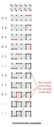
Suppose we are given a sequence of integer pairs, like (4, 3), (3, 8), etc. Each pair represents a connection between two sites. As we process these pairs, the connectivity of the graph changes. If a pair of sites is already connected, we ignore it, like (8, 9) in the example above.
Applications of Dynamic Connectivity
- Network Connectivity: If each integer in a pair represents a network node, the pair indicates that these two nodes should be connected. After building the dynamic connectivity graph, we can minimize wiring needs by ignoring connections between already-connected nodes.
- Variable Name Equivalence: Some programming environments allow declaring multiple variable names that refer to the same object (aliases). After a series of such declarations, the system needs to determine if two given variable names are equivalent.
- Mathematical Sets: At a higher level of abstraction, we can view the input integers as belonging to different mathematical sets. When processing a pair
p q, we are checking if they belong to the same set. If not, we merge the sets containingpandq.
Implementation
API and Framework
public class UF
{
    private int[] id;
    private int count;

    public UF(int N)
    {
        count = N;
        id = new int[N];
        for (int i = 0; i < N; i++)
            id[i] = i;
    }

    public int count() { return count; }

    public boolean connected(int p, int q) { return find(p) == find(q); }

    public int find(int p) { /* to be implemented */ }

    public void union(int p, int q) { /* to be implemented */ }

    public static void main(String[] args)
    {
        int N = StdIn.readInt();
        UF uf = new UF(N);
        while (!StdIn.isEmpty())
        {
            int p = StdIn.readInt();
            int q = StdIn.readInt();
            if (uf.connected(p, q))
                continue;
            uf.union(p, q);
            StdOut.println(p + " " + q);
        }
        StdOut.println(uf.count() + " components");
    }
}
int[] id: An array where the index represents a site, and the value is a component identifier.void union(int p, int q): Merges the components containing sitespandqif they are in different components.int find(int p): Returns the component identifier for the given site.boolean connected(int p, int q): Checks if two sites are in the same component.int count(): Returns the number of connected components.
quick-find Algorithm
We can use the value in id[p] as the identifier for the component containing site p. If id[p] == id[q], then p and q are connected. This requires that all sites in the same component have the same identifier.
int find(int p): Simply returnsid[p].void union(int p, int q): Ifpandqare not already connected, iterate through theidarray and change all entries withp’s identifier toq’s identifier.
public int find(int p) { return id[p]; }

public void union(int p, int q)
{
    int pID = find(p);
    int qID = find(q);

    if (pID == qID) return;

    for (int i = 0; i < id.length; i++)
        if (id[i] == pID) id[i] = qID;
    count--;
}
Analysis: In
quick-find, thefind()operation is very fast (constant time), butunion()must scan the entire array. For large-scale problems, this is inefficient, with a time complexity of approximately (O(N^2)).
quick-union Algorithm
Instead of ensuring all sites in a component share the same identifier, we can represent components using links. Each entry id[p] points to another site in the same component, forming a tree-like structure. The root of a tree is a site that points to itself (id[k] == k).
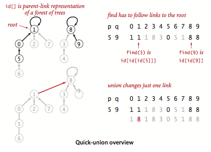
int find(int p): Follows the links frompto find its root.void union(int p, int q): Finds the roots ofpandqand makes one root point to the other.
private int find(int p)
{
    while (p != id[p])
        p = id[p];
    return p;
}

public void union(int p, int q)
{
    int pRoot = find(p);
    int qRoot = find(q);
    if (pRoot == qRoot) return;
    id[pRoot] = qRoot;
    count--;
}
Analysis: The performance of
quick-unionis highly dependent on the input. In the best case, its time complexity can be linear. In the worst case, the trees can become very tall, leading to (O(N^2)) complexity. Overall, whilequick-unionis not guaranteed to be faster thanquick-findin every case, it is generally an improvement.
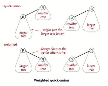
Weighted quick-union Algorithm
The main performance issue with quick-union is that the trees can become excessively deep. This often happens when a large tree is linked to a small one. We can avoid this by keeping track of the size of each tree and always linking the root of the smaller tree to the root of the larger tree. This is the weighted quick-union algorithm.
We need an extra array sz to store the size of each component.
public class WeightedQuickUnionUF
{
    private int[] id;
    private int[] sz;
    private int count;

    public WeightedQuickUnionUF(int N)
    {
        count = N;
        id = new int[N];
        sz = new int[N];
        for (int i = 0; i < N; i++)
        {
            id[i] = i;
            sz[i] = 1;
        }
    }

    public int count() { return count; }

    public boolean connected(int p, int q){ return find(p) == find(q); }

    private int find(int p)
    {
        while (p != id[p])
            p = id[p];
        return p;
    }

    public void union(int p, int q)
    {
        int pRoot = find(p);
        int qRoot = find(q);
        if (pRoot == qRoot) return;

        // Make smaller root point to larger one
        if (sz[pRoot] < sz[qRoot])
        {
            id[pRoot] = qRoot;
            sz[qRoot] += sz[pRoot];
        }
        else
        {
            id[qRoot] = pRoot;
            sz[pRoot] += sz[qRoot];
        }
        count--;
    }
    // main method remains the same
}
Analysis: The time complexity of the weighted
quick-unionalgorithm is proportional to (\log N). It is the only one of the three algorithms suitable for solving large-scale practical problems.
Why use component size instead of height as the weight?
- Because of how the trees are structured in union-find, the height of a tree will never be greater than (\log_2 N) of its size. Using size is sufficient and has a negligible impact on performance compared to height.
- Tracking tree size is easier, especially when path compression is used. Path compression can change the tree’s structure and height, making height difficult to track accurately.
Optimal Algorithm: Path Compression
Although the weighted quick-union algorithm is already very efficient, there is still room for improvement. Path compression is an easy-to-implement and highly effective optimization. The idea is simple: since we want to keep the trees as flat as possible, we can make every node on the path to the root point directly to the root.
We can add another loop to find() to achieve this:
private int find(int p)
{
    int root = p;
    // Find the root
    while (root != id[root])
        root = id[root];
    // Link all nodes on the path to the root
    while (p != root)
    {
        int next = id[p];
        id[p] = root;
        p = next;
    }
    return root;
}
This method is simple and effective, producing trees that are nearly flat. It is difficult to improve upon the weighted quick-union algorithm with path compression in practice.
The weighted quick-union algorithm with path compression is the optimal algorithm for solving the dynamic connectivity problem. Its amortized time complexity is nearly constant.